European Journal of Scientific Research - EuroJournals

Robust Control of a Doubly Fed Asynchronous Machine of a Wind Turbine System 799
⎡ Rr
M ⎢
L
= − ⋅ ⎢ r
Lr
⎢ w
⎢
⎣
⎤
w ⎥
⎥
Rr
− ⎥
L ⎥ r ⎦
C ,
⎡ 2
M
⎢Rs
+ ⋅ R
2
= ⎢ L
D
r
⎢
⎢ σ ⋅ Ls.
W
⎢⎣
r
− σ ⋅ L . W
M
Rs
+
L
III. The H∞ Controller Design Method
It is necessary to recall the basics of a control loop (fig.3), with: Δ m : is the system uncertainty, K: the
controller , G: the nominal system.
s
2
2
r
⋅ R
r
M
L
r
0
⎤
0 ⎥
⎥
M ⎥
⎥
Lr
⎥⎦
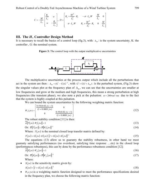
Figure 3: The control loop with the output multiplicative uncertainties
The multiplicative uncertainties at the process output which include all the perturbations that
' −1
act in the system are then : Δm = ( G − G).
G , with G′ = G(
I + Δ m ) : is the perturbed system, (Fig.3) show
the singular values plot at the frequency plan of Δ m , we can see that the uncertainties are smaller at
low frequencies and grow at the medium and high frequencies, this mean a strong perturbation at high
frequencies (the transient phase), we also note a pick at the pulsation: ω = 260rad / sec due to the fact
that the system is highly coupled at this pulsation.
We can bound the system uncertainties by the following weighting matrix function:
⎡ 0.
55(
0.
02 jw + 1)
⎢
( 1 + 0.
0001 jw)
( jw)
= ⎢
⎢ 0
⎢⎣
⎤
0 ⎥
⎥
0.
55(
0.
02 jw + 1)
⎥
( 1 + 0.
0001 jw)
⎥⎦
W t (12)
The robust stability condition [11] is then:
σ [ T ( jw)
⋅Wt
( jw)
] ≺ 1
(13)
Or: [ ( ) ] [ ( ) ] 1 −
σ T jw < σ Wt
jw
(14)
Where: T ( jw)
is the nominal closed loop transfer matrix defined by:
( ) ( ) ( ) [ ( ) ( ) ] 1 −
T jw = G jw ⋅ K jw ⋅ I + G jw ⋅ K jw
(15)
The equations (13) allow us to guaranty the stability robustness, in other hand we most
guaranty satisfying performances (no overshoot, satisfying time response …etc) in the closed loop
(performances robustness), this can by done by the performance robustness condition [12]:
σ [ S( jw)
⋅W
p ( jw)
] ≺ 1
(16)
Or: [ ( ) ] [ ( ) ] 1 −
σ S jw < σ Wp
jw
(17)
Where:
• S ( jw)
is the sensitivity matrix given by:
( ) [ ( ) ( ) ] 1 −
S jw = I + G jw ⋅ K jw
(18)
• WP ( jw)
is a weighting matrix function designed to meet the performance specifications desired
in the frequency plan, we choose the following matrix function: