State of the Bay Report 2010-Final - Anchor Environmental
State of the Bay Report 2010-Final - Anchor Environmental
State of the Bay Report 2010-Final - Anchor Environmental

You also want an ePaper? Increase the reach of your titles
YUMPU automatically turns print PDFs into web optimized ePapers that Google loves.
<strong>the</strong>se species usually provide <strong>the</strong> largest contribution to biomass. Smaller r-selected, opportunistic<br />
species with a shorter life-span are also represented, and usually dominate numerically but make a<br />
small (<strong>of</strong>ten insignificant) contribution to overall biomass (Warwick 1993). However, in an area<br />
affected by pollution (or some o<strong>the</strong>r form <strong>of</strong> disturbance), <strong>the</strong> large and long-lived (k-selected)<br />
species are less favoured and opportunistic (r-selected) species eventually become dominant in both<br />
biomass and numbers. When cumulative contributions by species to overall abundance and biomass<br />
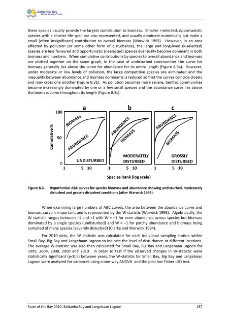
are plotted toge<strong>the</strong>r on <strong>the</strong> same graph, in <strong>the</strong> case <strong>of</strong> undisturbed communities <strong>the</strong> curve for<br />
biomass generally lies above <strong>the</strong> curve for abundance for its entire length (Figure 8.3a). However,<br />
under moderate or low levels <strong>of</strong> pollution, <strong>the</strong> large competitive species are eliminated and <strong>the</strong><br />
inequality between abundance and biomass dominants is reduced so that <strong>the</strong> curves coincide closely<br />
and may cross one ano<strong>the</strong>r (Figure 8.3b). As pollution becomes more severe, benthic communities<br />
become increasingly dominated by one or a few small species and <strong>the</strong> abundance curve lies above<br />
<strong>the</strong> biomass curve throughout its length (Figure 8.3c).<br />
Cumulative %<br />
100<br />
50<br />
0<br />
UNDISTURBED<br />
1 5 10<br />
a b c<br />
MODERATELY<br />
DISTURBED<br />
GROSSLY<br />
DISTURBED<br />
1 5 10 1 5 10<br />
Species Rank (log scale)<br />
Figure 8.3. Hypo<strong>the</strong>tical ABC curves for species biomass and abundance showing undisturbed, moderately<br />
disturbed and grossly disturbed conditions (after Warwick 1993).<br />
When examining large numbers <strong>of</strong> ABC curves, <strong>the</strong> area between <strong>the</strong> abundance curve and<br />
biomass curve is important, and is represented by <strong>the</strong> W statistic (Warwick 1993). Algebraically, <strong>the</strong><br />
W statistic ranges between –1 and +1 with W = +1 for even abundance across species but biomass<br />
dominated by a single species (undisturbed) and W = –1 for patchy abundance and biomass being<br />
compiled <strong>of</strong> many species (severely disturbed) (Clarke and Warwick 1994).<br />
For <strong>2010</strong> data, <strong>the</strong> W statistic was calculated for each individual sampling station within<br />
Small <strong>Bay</strong>, Big <strong>Bay</strong> and Langebaan Lagoon to indicate <strong>the</strong> level <strong>of</strong> disturbance at different locations.<br />
The average W-statistic was also <strong>the</strong>n calculated for Small <strong>Bay</strong>, Big <strong>Bay</strong> and Langebaan Lagoon for<br />
1999, 2004, 2008, 2009 and <strong>2010</strong>. In order to test if <strong>the</strong> observed changes in W-statistic were<br />
statistically significant (p