RESEARCH· ·1970·

where
V=volume, and
t =time.
And, for small increments of time (at),
av
aQ=-. (3)
at
If we substitute in equation 1 and rearrange,
aV=T·iLat. (4)
Where artesian conditions apply, Tis constant. Therefore,
if we assume a unit width,
aVociat. (5)
We cn,nnot actually determine ~ V for our site from
equ~ttion 4 as we do not know T. However, using equatiOij.
·5 n.t some point in our section we can com·pute
the. gradient, plot it versus time, and then mechanically
integrate the graph and use it to determine the direction
of fiow, the time at which bank storage begins, and the
time at which n.n equivalent volume has left the bank.
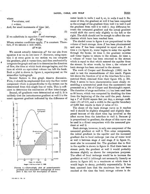
Such a plot is shown in figure 4, superimposed on the
streamflow hydrograph.
Several factors in this graph deserve discussion.
First, it should be emphasized that only the flow vector
componerit which is perpendicular to the stream can be
determined from this single line of wells. This is sufficient
to determine the mechanis1n of flow interchange.
Second, all gradients were determined at well 2. It is
~mlikely that the instantaneous gradient at well 2 is the
exact apparent gradient indicated by the difference of
1 6
X
0
z
8 5
w
(/)
0:
w
0.. 4
...
w
u..
u
iii 3
::::l
u
~
0 20 40 60 80
TIME, IN HOURS
Began 1700 hours April 3, 1968
)rrouum 4.~Chronologic
c
DANIEL, CABLE, AND WOLF
-0.010 ...
z
w
Ci
<
0:
-0.005
(.!)
u
0:
...
w
0
:E
0
i=
z
w
...
0
+0.005 0..
+0.010
100
plot of potentiometric
g·radient and streamflow hydrograph of storm
peak 3. See text for description of letters.
B221
water levels in wells 1 and 2, or, in wells 2 and 3. Because
of this, the gradient at well 2 has been computed
as the average of the gradient from well1 to well2 and
the gradient from well 2 to well 3. Any difference between
the computed gradient and the actual grad·ient
would shift the curve only slightly to the left or the
right. The shift should not be enough to affect the conclusions
which have been reached here.
The shaded areas in figure 4 are proportional to the
volume of bank storage. Area X has been planimetered
and ·area Y has been computed to equal area X. At
time a (in figure 4), water begins to enter the aquifer
through the banks. At time b, the gradient reverses
and water begins to return to the stream. At time o,
a volume of water has been returned to the stream
which is equal to that which entered the aquifer from
the stream. In other words, by time o, the volume of
bank storage has been returned to the stream.
The work of Cooper and Rorabaugh ( 1963) can be
used to test the reasonableness of this .result. Figure
5iii shows the function of Q at the interface for a symmetrical
flood, obtained from their figure 102, p. 361.
Peak 3 seems to have characteristics more closely resembling
a symmetrical peak than the asymmetric one
presented on p. 364 of Cooper and Rorabaugh's report.
The duration of stage oscillation ( 7') has been used here
as 80 hours, which was computed by doubling the time
from the beginning of the rise until the peak. Assuming
a T of 30,000 square :feet per day, a storage coefficient
(S) of 0.01, and a width to the aquifer boundary
o:f 6,000 :feet results in their f3 value of 0.1.
The shape o:f the bank storage curve as it reaches
well 2 should be slightly elongated and slightly dampened
because of the short time lag in·volved as the
effect moves from the interface to well 2. Because Q
is proportional to gradient, the shape o:f this curve can
be used in a dire~t comparison with the measured gradient
at well 2. ·
Bank storage, hmvever, is only, one component o:f the
measured gradient at well 2. Two other components,
the initial gradient in the aquifer and the increased
gradient due to local recharge (see rise o:f water level
at well 4 'between stage A and stage B in figure 3),
must also be accounted for. The gradient due to flo~
in the aquifer is shown in figure 5i. Had there been no
stream peak, the gradient at well · 2 would probably
decrease slightly as shown for comparison purposes.
The effect of local recharge would . be to increase the
gradient at well 2 (although not ne~essarily linearly as
shown iri figu~e 5ii) to a maximuin at which time it
would begin to decay, probably exponentially. It has
been assumed here that the maximum has not been
reached at th~ time the h~nk. storage volume is de-
372-400 0- 70- 16