Archaeoseismology and Palaeoseismology in the Alpine ... - Tierra

More documents

Recommendations

Info

Furthermore this region in central Greece undergoes a rapid main extension in N‐S direction with approximately 6‐15 mm/a (Kokkalas et al., 2007b). The Kaparelli fault is an active normal limestone fault scarp with a height of about 3 ‐ 5 m. The last major earthquake occurred in winter 1981. Three events with magnitudes greater than 6 were measured. During the night of the 24 th ‐25 th February the fist two events had a magnitude of 6.7 and 6.4 and the third event on the 4 th March reached magnitude 6.3 (Hubert et al., 1996). After those events 2‐ D roughness analyses (Stewart, 1996), cosmogenic dating (Benedetti et al., 2003), trenching (Kokkalas et al., 2007) and deformation monitoring by using a dense network of Fig. 3: A) The southern segment of the Kaparelli fault. B) One scan position and the scarp layout non‐permanent GPS stations and extensometers (Ganas et al. 2007) have been carried out especially on the Kaparelli fault. Benedetti et al. (2003) assumed three events from his cosmogenic dating. The results give evidence for events at 20±3 ka, 14.5±0.5 ka and 10.5±0.5 ka. According to that the time intervals between slip events are 3000‐9000 years, 4000‐5000 years and 10000‐ 11000 years. Kokkalas et al. (2007) results of the trench show again three events at around 7.5 ka, 5.8 ka and 1.4 ka. So that now seven events include the 1981 earthquake are proposed FUNDAMENTALS OF LIDAR The terrestrial laser scanning (TLS) was established as a good data acquisition in geoscience and geological engineering in difficult accessible areas. As the TLS has a high spatial and temporal resolution it is an effective remote sensing technology for reconstruction, monitoring and observation of mass movement phenomena and related hazards. The raw point cloud dataset includes the distance between object and TLS, the x‐, y‐ and z‐ coordinates and the received intensity. With the integrated digital camera the panchromatic information is recorded. Furthermore, the working capabilities of TLS in geosciences are based in the area‐measured data in safety range (> 600m). Successful investigations in geosciences with TLS were published by e.g. Kuhn & Prüfer (2007) for mass movement observation on the island Rügen, Travelletti et al. (2008) for landslide monitoring, Rabatel et. al. (2008) for mass balance of rockfall in the Alps or by Slob et. al. (2007) for fracture systems. The fundamental principle of LiDAR (Light 1 st INQUA‐IGCP‐567 International Workshop on Earthquake Archaeology and Palaeoseismology 170 Detection And Ranging) is to generate coherent laser beam with little beam divergence by stimulated emission. The electromagnetic waves are reflected by surfaces and the receiver detects portions of the backscattered signal. Fig. 4: The terrestrial laser scanner ILRIS 3D from Optech in the field The laser ranging system is based on measuring the time‐ of‐flight of the short laser signal. The range or distance to the target is calculated from the time elapse of the pulse between the transmitter and receiver, and, the speed of the laser pulse. For the pulse detection the first pulse, the last pulse or the strongest pulse can be selected. In our case we used the TLS ILRIS‐3D from Optech Inc., Ontario, CA (Fig.4). The technical Data of ILRIS‐3D show table1. Table 1: Technical Data Data sampling rate 2500 points per sec. Beam divergence 0.00974° Minimum spot step 0.00115° Laser wavelength 1500nm Raw range accurancy 7mm @ 100m Raw positional accurancy 8mm @ 100m Digital camera Integrated digital camera Scanner field of view 40° x 40° DATA ACQUISITION AND FIRST RESULTS Major aims of the investigation were to find quantitative and qualitative data for the reconstruction of surfaces and to analyze the tectonic geomorphology and paleoseismology of active faults with TLS to reconstruct fault history and activity along surface rupturing scarps. In this context, the detailed structural analysis of rock surfaces is fundamental and can be realized by a HRDEM. The scarp surface was scanned where Benedetti et al. (2003) took samples for the cosmogenic dating method (Fig. 3B). For high quality data, the terrestrial laser scanner should detect the object from different points of view. Hence a relative complete point cloud can be produced. In this case we have four scan positions with eleven scan windows for the circa 35m long scarp. The density of points by the scans ranges between 1mm to 5.1mm. The scan sequence is composed of approximately 94 million points.
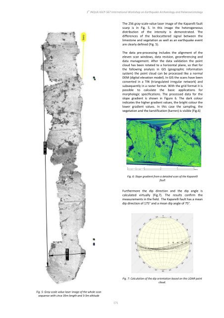
Fig. 5: Gray‐scale value laser image of the whole scan sequence with circa 35m length and 3‐5m altitude 1 st INQUA‐IGCP‐567 International Workshop on Earthquake Archaeology and Palaeoseismology 171 The 256 gray‐scale‐value laser image of the Kaparelli fault scarp is in Fig. 5. In this image the heterogeneous distribution of the intensity is demonstrated. The differences of the backscattered signal between the limestone and vegetation as well as an earthquake event are clearly defined (Fig. 5). The data pre‐processing includes the alignment of the eleven scan windows, data revision, georeferencing and data management. After the data validation the point cloud has been rotated to a horizontal plane, so that for the following analysis in GIS (geographic information system) the point cloud can be processed like a normal DEM (digital elevation model). In GIS the scans have been converted in a TIN (triangulated irregular network) and subsequently in a raster format. With the grid format it is possible to calculate the basic applications for morphologic specifications. The processed data for the slope gradient is shown in Figure 6. The dark colour indicates the higher gradient values, the bright colour the lower gradient values. In this case the sampling, the vegetation and the karstification (karren) is visible (Fig.6) Fig. 6: Slope gradient from a detailed scan of the Kaparelli fault Furthermore the dip direction and the dip angle is calculated virtually (Fig.7). The results confirm the measurements in the field. The Kaparelli fault has a mean dip direction of 175° and a mean dip angle of 75°. Fig. 7: Calculation of the dip orientation based on the LiDAR point cloud.
Page 1:
Abstracts Volume Archaeoseismology
Page 4 and 5:
Edita e imprime: Sección de Public
Page 7 and 8:
1 st INQUA‐IGCP‐567 Internation
Page 9 and 10:
the importance of performing absolu
Page 11 and 12:
indicative of strike‐slip faultin
Page 13 and 14:
DISCUSSION Based on detailed field
Page 15 and 16:
Table 1: Source parameters used in
Page 17 and 18:
elations. However, the attenuation
Page 19 and 20:
mostly concentrated on the DST in I
Page 21 and 22:
continuous support. N. Shalev, G. G
Page 23 and 24:
The tumulus initial morphology show
Page 25 and 26:
Page 27 and 28:
our understanding and prediction of
Page 29 and 30:
spans, with a threefold increase fr
Page 31 and 32:
Nevertheless the lack of research,
Page 33 and 34:
earthquake. In uncertain cases, as
Page 35 and 36:
The site reconnaissance successfull
Page 37 and 38:
Page 39 and 40:
Page 41 and 42:
Page 43 and 44:
Table 1: Surface faulting extent re
Page 45 and 46:
Page 47 and 48:
The graben has a markedly asymmetri
Page 49 and 50:
Page 51 and 52:
Page 53 and 54:
are a valuable addition to the rout
Page 55 and 56:
to 400 m) the calculated values for
Page 57 and 58:
RISK ANALYSIS The created hazard ma
Page 59 and 60:
290 m water depth the basin accumul
Page 61 and 62:
CONCLUSIONS From the palaeostress a
Page 63 and 64:
Fig. 2: Geological map of the study
Page 65 and 66:
Page 67 and 68:
Page 69 and 70:
Page 71 and 72:
however, the massive 1995 earthquak
Page 73 and 74:
mapped on the slopes above Qiryat
Page 75 and 76:
Page 77 and 78:
interpreted as either an expression
Page 79 and 80:
The Shepran Cave is located on the
Page 81 and 82:
Page 83 and 84:
Page 85 and 86:
Page 87 and 88:
properties. The mean value of speci
Page 89 and 90:
Page 91 and 92:
excavated a deep trench, thus provi
Page 93 and 94:
Page 95 and 96:
Page 97 and 98:
Page 99 and 100:
Fig. 8: Seismic ground shaking may
Page 101 and 102:
elevant qualitative criteria are po
Page 103 and 104:
CONCLUDING REMARKS The exposed exam
Page 105 and 106:
produced by significantly different
Page 107 and 108:
It is possible that a portion of th
Page 109 and 110:
In addition, the Database of histor
Page 111 and 112:
were published by IGME (1983) and E
Page 113 and 114:
Page 115 and 116:
The city collapsed and it was aband
Page 117 and 118:
Page 119 and 120:
Fig. 4: Slipped lintel in a window
Page 121 and 122: to overcome shear resistance and in
Page 123 and 124: Newmark, N.M. (1965). Effects of ea
Page 125 and 126: associated with various tsunamis (<
Page 127 and 128: 1 st INQUA‐IGCP‐567 Internation
Page 129 and 130: this method, the magnitude of the e
Page 133 and 134: etween pieces. Fragments have not f
Page 137 and 138: on the exact date of the earthquake
Page 139 and 140: THE ARCHAEOLOGICAL ZONE COLOGNE Aft
Page 143 and 144: affecting the Alcázar was about 50
Page 147 and 148: archaeoseismology could instead bec
Page 149 and 150: In the area later occupied by Vilni
Page 155 and 156: Fig. 2: Assemblage of landforms ass
Page 157 and 158: Fig. 8: Data and regression for mag
Page 159 and 160: Fig. 3: Relationships among magnitu
Page 161 and 162: CONCLUSIONS 1. Spatial distribution
Page 163 and 164: The stratigraphic sequence (Fig. 4)
Page 165 and 166: especially in the zones of hanging
Page 169 and 170: interpretations are based on relati
Page 171: 1 st INQUA‐IGCP‐567 Internation
Page 177 and 178: (~40 cm), F‐ rotated building str
Page 179 and 180: Index 1 st INQUA‐IGCP‐567 Inter
Page 181: 1 st INQUA‐IGCP‐567 Internation
show all

Archaeoseismology and Palaeoseismology in the Alpine ... - Tierra

You also want an ePaper? Increase the reach of your titles

Delete template?

Save as template?