Spectral Theory in Hilbert Space

92 13. FIRST ORDER SYSTEMS
Since W is assumed locally integrable it is clear that constant n ×
1 matrices are locally in L2 W so (each components of) W u is locally
integrable if u ∈ L2 W . It is also clear that u and ũ are two different
representatives of the same equivalence class in L2 W precisely if W u =
W ũ almost everywhere (Exercise 13.1).
Example 13.3. Any standard scalar differential equation may be
written on the form (13.1) with a constant, skew-Hermitian J. If it
is possible to do this so that Q and W are Hermitian, the differential
equation is called formally symmetric. We have already seen this in
the case of the Sturm-Liouville equation (10.1), which will be formally
symmetric if p, q and w are real-valued. The first order scalar equation
iu ′ + qu = wv is already of the proper form and formally symmetric if
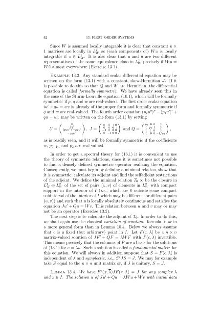
q and w are real-valued. The fourth order equation (p2u ′′ ) ′′ − (p1u ′ ) ′ +
qu = wv may be written on the form (13.1) by setting
U =
, J =
and Q =
u
hu ′
(p2u ′′ ) ′ −p1u ′
−p2u ′′
0 0 1 0
0 0 0 1
−1 0 0 0
0 −1 0 0
p0 0 0 0
0 p1 1 0
0 1 0 0
0 0 0 −1/p2
as is readily seen, and it will be formally symmetric if the coefficients
w, p0, p1 and p2 are real-valued.
In order to get a spectral theory for (13.1) it is convenient to use
the theory of symmetric relations, since it is sometimes not possible
to find a densely defined symmetric operator realizing the equation.
Consequently, we must begin by defining a minimal relation, show that
it is symmetric, calculate its adjoint and find the selfadjoint restrictions
of the adjoint. We define the minimal relation T0 to be the closure in
L 2 W ⊕ L2 W of the set of pairs (u, v) of elements in L2 W
,
with compact
support in the interior of I (i.e., which are 0 outside some compact
subinterval of the interior of I which may be different for different pairs
(u, v)) and such that u is locally absolutely continuous and satisfies the
equation Ju ′ + Qu = W v. This relation between u and v may or may
not be an operator (Exercise 13.2).
The next step is to calculate the adjoint of T0. In order to do this,
we shall again use the classical variation of constants formula, now in
a more general form than in Lemma 10.4. Below we always assume
that c is a fixed (but arbitrary) point in I. Let F (x, λ) be a n × n
matrix-valued solution of JF ′ + QF = λW F with F (c, λ) invertible.
This means precisely that the columns of F are a basis for the solutions
of (13.1) for v = λu. Such a solution is called a fundamental matrix for
this equation. We will always in addition suppose that S = F (c, λ) is
independent of λ and symplectic, i.e., S ∗ JS = J. We may for example
take S equal to the n × n unit matrix or, if J is unitary, S = J.
Lemma 13.4. We have F ∗ (x, λ)JF (x, λ) = J for any complex λ
and x ∈ I. The solution u of Ju ′ + Qu = λW u + W v with initial data