- Page 1:
Proceedings e report 90
- Page 4 and 5:
ECOS 2012 : the 25 th International
- Page 7 and 8:
Advisory Committee (Track Organizer
- Page 10 and 11:
The 25 th ECOS Conference 1987-2012
- Page 12 and 13:
VOLUME VI CONTENT VI. 1 CARBON CAPT
- Page 14 and 15:
-----------------------------------
- Page 16 and 17:
» Personal transportation energy c
- Page 18 and 19:
» Excess enthalpies of second gene
- Page 20 and 21:
VOLUME IV IV . 1 - FLUID DYNAMICS A
- Page 22 and 23:
» Exergy analysis and genetic algo
- Page 24 and 25:
» Optimal lighting control strateg
- Page 26 and 27:
» Stability and limit cycles in an
- Page 28 and 29:
PROCEEDINGS OF ECOS 2012 - THE 25 T
- Page 30 and 31:
Fig. 2. The exergy destruction of M
- Page 32 and 33:
ineffectiveness of the catalyst, in
- Page 34 and 35:
[ P EXmth EX SNG] ESR F where EXm
- Page 36 and 37:
Fuel inputkW 728221 203771 237719 3
- Page 38 and 39:
Not only at desined Rc (the ratio o
- Page 40 and 41:
4. DISCUSSION The graphic exergy an
- Page 42 and 43:
Figure 9(a) illustrates the energy
- Page 44 and 45:
Engineering Technical Conferences &
- Page 46 and 47:
generally there are four kinds of m
- Page 48 and 49:
However, even under the off-design
- Page 50 and 51:
Fig. 3. 600MW supercritical coal-fi
- Page 52 and 53:
CO2 rich loading(molCO2/molMEA) 0.4
- Page 54 and 55:
Net efficiency (%) 40.28 30.29 26.4
- Page 56 and 57:
Fig. 11. Schematic diagram of heat
- Page 58 and 59:
28.67%. In addition, through heat i
- Page 60 and 61:
Applied Thermal Engineering 2010;30
- Page 62 and 63:
Abstract: PROCEEDINGS OF ECOS 2012
- Page 64 and 65:
Fig. 1. Solution diagram of „four
- Page 66 and 67:
K ~ K 1 eK 1a p K 1a iK mK
- Page 68 and 69:
Oxygen recovery rate, % 105 95 85 7
- Page 70 and 71:
Calculated optimal compressor press
- Page 72 and 73:
PROCEEDINGS OF ECOS 2012 - THE 25 T
- Page 74 and 75:
The net amount of the flue gas leav
- Page 76 and 77:
Figure 3. Idea for lignite drying b
- Page 78 and 79:
Energy efficiency, % 34,00 33,00 32
- Page 80 and 81:
points efficiency increase related
- Page 82 and 83:
Figure A1b. Thermoflex flow sheet o
- Page 84 and 85:
Figure A3a. Thermoflex flow sheet o
- Page 86 and 87:
Figure A4. Thermoflex flow sheet of
- Page 88 and 89:
Abstract: PROCEEDINGS OF ECOS 2012
- Page 90 and 91:
2.1. Life Cycle Assessment 2.1.1. G
- Page 92 and 93:
these factors. A sensitivity analys
- Page 94 and 95:
methane slip contributes to 13% of
- Page 96 and 97:
As can be seen in Fig. 5 the impact
- Page 98 and 99:
References [1] Eurobserv’er, The
- Page 100 and 101:
PROCEEDINGS OF ECOS 2012 - THE 25 T
- Page 102 and 103:
in which CO2 is separated from H2,
- Page 104 and 105:
dimensions of water droplets and wa
- Page 106 and 107:
Temperature (°C) 8 7 6 5 4 3 2 1 0
- Page 108 and 109:
4. Conclusions In the present paper
- Page 110 and 111:
Abstract: PROCEEDINGS OF ECOS 2012
- Page 112 and 113:
penalty, but without separate captu
- Page 114 and 115:
0.5 - 0.7 kg/kg, resulting typicall
- Page 116 and 117:
3.3 - Utilising waste heat All exis
- Page 118 and 119:
4.5 - Suomusjärvi olivine deposits
- Page 120 and 121:
material will change from a few % t
- Page 122 and 123:
Fig. 5 Schematic diagram of the PFB
- Page 124 and 125:
8. Combined SO2 capture and CO2 min
- Page 126 and 127:
Fig. 10 Carbonate- (left) and sulph
- Page 128 and 129:
[13] Ekdahl, E., Idman, H. Statemen
- Page 130 and 131:
Abstract: PROCEEDINGS OF ECOS 2012
- Page 132 and 133:
HEAT Fig. 1. Scheme and main reacti
- Page 134:
(raw) materials pre-heating and AS
- Page 137 and 138:
Fig 3- Aspen Plus® model 110
- Page 139 and 140:
Table 4. Elemental and XRD analysis
- Page 141 and 142:
the ÅA CSM route. The content of M
- Page 143 and 144:
Abstract: PROCEEDINGS OF ECOS 2012
- Page 145 and 146:
moisture - 0,2237 ash - 0,0876 LHV
- Page 147 and 148:
2.2 CFB plant For the current momen
- Page 149 and 150:
The CO2 emission factor which indic
- Page 151 and 152:
The CO2 emission factor calculated
- Page 153 and 154:
Appendix A Fig A.1. Simulation mode
- Page 155 and 156:
(b) Fig. A.2. Simulation model of C
- Page 157 and 158:
Table A.1. Calculated parameters at
- Page 159 and 160:
References [1] Pfaff I., Oexmann J.
- Page 161 and 162:
with a CC installation could be avo
- Page 163 and 164:
2.3. Basic CHP plant indices. The b
- Page 165 and 166:
3. Off-design calculations The main
- Page 167 and 168:
Fig. 6. CHP plant efficiency Fig. 7
- Page 169 and 170:
amount of steam delivered to the he
- Page 171 and 172:
[5] Lukowicz H., Mroncz M.: Analysi
- Page 173 and 174:
water removal is feasible by coolin
- Page 175 and 176:
Figure 2. Sketch of the suggested P
- Page 177 and 178:
a b Figure 5. a) Exergy balance of
- Page 179 and 180:
The basis of comparison of each met
- Page 181 and 182:
Figure 7a. Impact of S/CATR on PCU
- Page 183 and 184:
However, more energy duty is requir
- Page 185 and 186:
Abstract: PROCEEDINGS OF ECOS 2012
- Page 187 and 188:
3.1. JACOBIAN-ASPEN Interface ASPEN
- Page 189 and 190:
Fig. 3. Triple Pressure Bottoming S
- Page 191 and 192:
As seen from Table 1, the mass flow
- Page 193 and 194:
4. Conclusion Fig. 5. Partial Emiss
- Page 195 and 196:
[19] Yantovski E., Shokotov M., Sho
- Page 197 and 198:
investigation and the developing of
- Page 199 and 200:
University of L’Aquila and German
- Page 201 and 202:
hydrogen combustion technology at d
- Page 203 and 204:
eversibility of a pre-treated synth
- Page 205 and 206:
Fig. 1. TG curves collected for spe
- Page 207 and 208:
(see Fig 5). Carbon dioxide uptake
- Page 209 and 210:
period is reduced to the first 15 c
- Page 211 and 212:
CO2 capture capacity up to 150 th c
- Page 213 and 214:
the way for biogas utilisation is t
- Page 215 and 216:
projectand is described in the foll
- Page 217 and 218:
4. Pilot plant tests In order to de
- Page 219 and 220:
Concerning the absorption reaction,
- Page 221 and 222:
with Regeneration (AwR), consists i
- Page 223 and 224:
[25] Aspen Plus 2004.1. Cambridge,
- Page 225 and 226:
systems for fuel drying waste strea
- Page 227 and 228:
heated in a heat exchanger placed i
- Page 229 and 230:
Fig. 2. Lower heating value of fuel
- Page 231 and 232:
Acknowledgements The results presen
- Page 233 and 234:
large amount of CO2 [1,5-7]. APCr a
- Page 235 and 236:
N 1 i ( x x i n 1 m ) 2.3. Carbon
- Page 237 and 238:
DTA analysis of the untreated APCrs
- Page 239 and 240:
Table 4. Relative Error (%) of the
- Page 241 and 242:
CaO HCl CaCl H O 193kJ / mol (
- Page 243 and 244:
[1] M. Fernández Bertos, S.J.R. Si
- Page 245 and 246:
Abstract: PROCEEDINGS OF ECOS 2012
- Page 247 and 248:
2. Process development 2.1. Backgro
- Page 249 and 250:
to dissolve the chloride salts prec
- Page 251 and 252:
The remaining 25% (5 ml/min) of the
- Page 253 and 254:
Table 6. Experimental conversions o
- Page 255 and 256:
p p 1 1. 5 p H 1 1. 5 2O p mi
- Page 257 and 258:
Calculating from the Aspen Plus mod
- Page 259 and 260:
[11] Mattila, H.-P., Experimental s
- Page 261 and 262:
Mg2SiO4(s) + 2CO2(g) →2MgCO3(s) +
- Page 263 and 264:
(Mg/Fe) of the mineral rock, Mg-sil
- Page 265 and 266:
Figure 2. Effect of Mg/Fe ratio of
- Page 267 and 268:
Figure 4 shows that an increase in
- Page 269 and 270:
Figure 5. Process flow diagram of M
- Page 271 and 272:
2. Only cold utility is needed belo
- Page 273 and 274:
extraction process at 400 °C (~ 62
- Page 275 and 276:
Table A2. Extraction equations and
- Page 277 and 278:
[13] Teir S, Kuusik R, Fogelholm CJ
- Page 279 and 280:
In the area of coal technologies al
- Page 281 and 282:
Tabel 1. Characteristics quantities
- Page 283 and 284: N m eT 4a ~ T cp T4a 1 ( K
- Page 285 and 286: Auxiliary power rate of ASU, % 40 4
- Page 287 and 288: [8] Buhre B.J.P., Elliott L.K., She
- Page 289 and 290: 1.1 - Cement Manufacturing The ceme
- Page 291 and 292: 2. Numerical model The purpose of t
- Page 293 and 294: -0.309x15.77x2 2.085x3 240x4 12.53x
- Page 295 and 296: Table 4 - Results of the optimizati
- Page 297 and 298: PROCEEDINGS OF ECOS 2012 - THE 25 T
- Page 299 and 300: 1. Define the studied system (in th
- Page 301 and 302: cycle) or a lignin extraction plant
- Page 303 and 304: limiting factor for the maximum siz
- Page 305 and 306: Table 5. Key data for the four ener
- Page 307 and 308: Global CO 2 emissions [ktonnes/yr]
- Page 309 and 310: for biofuels and the investment cos
- Page 311 and 312: The possibility to capture CO2 from
- Page 313 and 314: [17] Berglin N, Andersson L. Proces
- Page 315 and 316: Therefore NL Agency (an agency of t
- Page 317 and 318: 2.2.2. Pinch analysis Pinch analysi
- Page 319 and 320: 3. Case study 3.1. Plant and proces
- Page 321 and 322: Te 1000 mp era 900 tur 800 e [°C 7
- Page 323 and 324: Application of the approach led to
- Page 325 and 326: The advantage of dynamic models is
- Page 327 and 328: e equal at both time intervals and
- Page 329 and 330: 2.5. Selecting the number of TSs Se
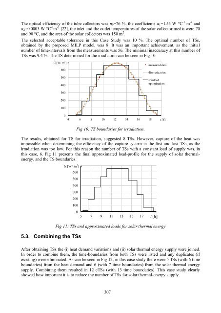
- Page 331 and 332: A) Time Slices for solar thermal en
- Page 333: The first step of procedure is to p
- Page 337 and 338: In the presented paper a framework
- Page 339 and 340: [5] Erdil E, Ilkan M, Egelioglu F.
- Page 341 and 342: PROCEEDINGS OF ECOS 2012 - THE 25 T
- Page 343 and 344: district energy network simulation
- Page 345 and 346: were decreased by 10°C.All scenari
- Page 347 and 348: Site 3 Heat sources Heat load Site
- Page 349 and 350: 3.2.2. Input data and assumptions A
- Page 351 and 352: Fig.7 shows the operation forecast
- Page 353 and 354: [13] TERMIS Operation User Guide, 7
- Page 355 and 356: Polygeneration is a term used to de
- Page 357 and 358: The increase in energy utilization
- Page 359 and 360: are available for an entire year, 8
- Page 361 and 362: 6. Extensions to core methodology 6
- Page 363 and 364: thermal storage and possible suppor
- Page 365 and 366: laterites. Ore Geology Reviews, v.
- Page 367 and 368: Abstract: PROCEEDINGS OF ECOS 2012
- Page 369 and 370: gasification [15], hybrid biomass g
- Page 371 and 372: the second reactor. In this unit, s
- Page 373 and 374: The variables effect was evaluated
- Page 375 and 376: atio, as well as the shift-syngas f
- Page 377 and 378: Fig. 4. Effect of operating tempera
- Page 379 and 380: SDG has slight effect on the syngas
- Page 381: [26.] Castle WF. Air separation and