View PDF Version - RePub - Erasmus Universiteit Rotterdam

Chapter 3.2
146
The correlation between single observations made on the same subject (between two
measurements of either the same marker or two different markers) is introduced by
specifying a joint distribution for bi =(b ′ i,1,...,b ′ i,R) ′ , the vector of i-th subject
specific random effects pertaining to all R markers. Particularly, the covariance
matrix var(bi) is assumed to be a general (unstructured) positive definite matrix D.
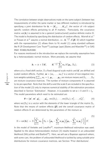
The model is finalized by specifying the distribution of random effects. Morrell et al. 7
or Fieuws et al. 9 assume a normal distribution, i.e., bi
i.i.d.
∼ N(β, D) which together
with the representation (2) allows them to fit model (1) using standard software
like R (R Development Core Team13 ) package lme4 (Bates and Maechler15 )orSAS
PROC MIXED/NLMIXED.
For reasons mentioned in the introduction we replace the normality assumption here
by a heteroscedastic normal mixture. More precisely, we assume that
bi = s + S b ∗ i , b ∗ i
i.i.d.
∼
K�
wk N (μk, Dk), (3)
where s is a fixed shift vector, S a fixed diagonal scale matrix and b ∗ i are shifted and
scaled random effects. Further, w =(w1,...,wK) ′ is a vector of non-negative mixture
weights satisfying �K k=1 wk =1,μ1,...,μK are mixture means and D1,...,DK
are mixture covariance matrices. The number of mixture components K is assumed
to be pre-specified. Note that the shift s and the scale S are included in the specification
of the model (3) only to improve numerical stability of the estimation procedure
described in Section ’Estimation’. However, it is possible to set s = 0 and S = Iq.
The model parameters which need to be estimated are
θ = � α ′ , w ′ , μ ′ 1,...,μ ′ K, vec(D1),...,vec(DK), σ 2 1,...,σ 2 � ′,
R (4)
where vec(Dk) is a vector with the elements of the lower triangle of the matrix Dk.
Note that the means of random effects (β) and the overall covariance matrix of
random effects D are determined by the parameters of the mixture as
D =var(bi) = S
� K�
k=1
wk
�
Dk +
�
μ k −
K�
j=1
k=1
wj μ j
��
μ k −
K�
j=1
wj μ j
� ′ � �
In the model of Verbeke and Lesaffre 10 , maximum-likelihood estimation was used.
Applied to the above heteroscedastic mixture (3) results however in an unbounded
likelihood (McLachlan and Basford16 ). Here, we will use a Bayesian approach where,
with some care, the problem of unbounded likelihood is tackled by using suitable prior
distributions for mixture covariance matrices, see Section ’Prior distributions’.
S ′ .
(5)