View PDF Version - RePub - Erasmus Universiteit Rotterdam

Dynamic prediction of response using longitudinal profi les 95
Results of the longitudinal prediction with the indirect approach
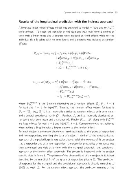
A bivariate linear mixed effects model was designed to model = load and ln(ALT )
simultaneous. To catch the behavior of the load and ALT over time B-splines of
time with 5 inner knots and 3 degrees were included as fixed effects while for the
individual fit a B-spline with no inner knots and 2 degrees was included as random
effects:
where B l,random
2,0,i
Y1,i,j = loadi,j = β 1 1 + β 1 2sexi + β 1 3age i + β 1 4PrRxi
+ β 1 5geno i,B + β 1 6geno i,C + β 1 7geno i,D
+ B
1,f ixed
3,5 (ti,j)
+ b 1 0,i + B 1,random
2,0,i (ti,j)+ε 1 i,j
Y2,i,j = ln(alt)i,j = β 2 1 + β 2 2sexi + β 2 3age i + β 2 4PrRxi
+ β 2 5geno i,B + β 2 6geno i,C + β 2 7geno i,D
+ B
2,f ixed
3,5 (ti,j)
+ b 2 0,i + B 2,random
2,0,i (ti,j)+ε 2 i,j
is the B-spline depending on 2 random effects bl 1,i ,bl 2,i , l = 1
for load and l = 2 for ln(ALT). That is, the random effect vector for load is
b 1 i =(b 1 0,i ,b1 2,i ,b1 3,i )′ , i.i.d. normally distributed random effects with zero mean
and a general covariance matrix D1 . Further, εl i,j are i.i.d. normally distributed er-
ror terms with zero mean and a variance σ2 l . Finally, βl 1 ,...,βl 7
are fixed effects for load, l = 1 and ln(ALT), l = 2. Convergence was not achieved
along with Bl,f ixed
3,5
when adding a B-spline with a higher degree to the random effect.
For each subject i the model above was fitted separately to the group of responders
and non-responders, omitting the data of subject i, similar to the cross-validated
approach of the pooled logistic regression above. With the two sets of fit per subject
- as a responder and as a non-responder - the posterior probability of response was
then calculated one visit at a time with the marginal approach, the conditional
approach or the random effect approach. The process is illustrated with the subject
specific plots in figure 3. The pattern of the observed load of the subject in 3a is best
described by the marginal fit of the group of responders (figure 2). The prediction
of response for the marginal and the conditional approach is already emerging to
100% at week 16. For the random effect approach the prediction remains at the