View PDF Version - RePub - Erasmus Universiteit Rotterdam
View PDF Version - RePub - Erasmus Universiteit Rotterdam
View PDF Version - RePub - Erasmus Universiteit Rotterdam

Create successful ePaper yourself
Turn your PDF publications into a flip-book with our unique Google optimized e-Paper software.
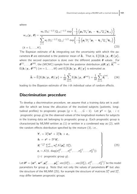
where<br />
wi,k(y i, θ) =<br />
(k =1,...,K).<br />
wk |Dk| −1/2 |Qi,k| −1/2 �<br />
exp − 1<br />
K�<br />
wj |Dj|<br />
j=1<br />
−1/2 |Qi,j| −1/2 exp<br />
Discriminant analysis using a MLMM with a normal mixture 151<br />
�<br />
′ −1<br />
μk Dk μ ′ −1<br />
k − ηi,k Qi,kη �<br />
i,k<br />
�<br />
2<br />
�<br />
− 1<br />
�<br />
′ −1<br />
μj Dj 2<br />
μ ′ −1<br />
j − ηi,j Qi,j η �<br />
i,j<br />
�<br />
(23)<br />
The Bayesian estimate of bi integrating out the uncertainty with which the pa-<br />
rameters θ are estimated is the posterior mean of � bi. That is, E � E(bi | y i, θ) � � y � ,<br />
where the second expectation is done over the different possible θ values. For<br />
θ (1) ,...,θ (M) , the (MCMC) sample from the posterior distribution p(θ | y), � b (m)<br />
i =<br />
E(bi | y i, θ (m) )(m =1,...,M)andE � E(bi | y i, θ) � �<br />
� y is estimated as<br />
�bi = � E � E(bi | y i, θ) � � y � = 1<br />
M<br />
M�<br />
E � �<br />
bi<br />
� y i, θ (m)� = 1<br />
M<br />
m=1<br />
M�<br />
m=1<br />
�b (m)<br />
i , (24)<br />
leading to the Bayesian estimate of the i-th individual value of random effects.<br />
Discrimination procedure<br />
To develop a discrimination procedure, we assume that a training data set is available<br />
for which we know the allocation of the involved subjects (patients, longitudinal<br />
profiles) to prognostic groups (g =0,...,G − 1). Let y g = {y i : i ∈<br />
prognostic group g} be the observed values of the longitudinal markers for subjects<br />
in the training data set belonging to prognostic group g. Each prognostic group is<br />
characterized by MLMM written as (1) or written in a condensed way as (2), with<br />
the random effects distribution specified by the mixture (3), i.e.,<br />
Y i = X g<br />
i αg + Z g<br />
i bi<br />
⎫<br />
+ εi,<br />
bi = s g + S g b ∗ i ,<br />
b ∗ i<br />
i.i.d.<br />
∼ � K<br />
k=1<br />
w g<br />
k<br />
εi ∼N(0, diag(σ g<br />
1<br />
N (μg k , Dg<br />
k ),<br />
2 ,...,σ g<br />
1<br />
(i ∈ prognostic group g).<br />
2 ,...,σ g<br />
R<br />
2 g 2<br />
,...,σR ))<br />
⎪⎬<br />
⎪⎭<br />
(25)<br />
Let θ g = � αg′ , w g′ , μ g′<br />
g ′ g<br />
1 ,...,μK , vec(D1 ),...,vec(Dg K ),σg<br />
2 g 2<br />
1 ,...,σR � ′<br />
be the model<br />
parameters for group g. Note that not only the values of parameters θ g but also<br />
the structure of the MLMM (25), for example the structure of matrices X g<br />
i and Zg<br />
i ,<br />
may differ between prognostic groups.