View PDF Version - RePub - Erasmus Universiteit Rotterdam

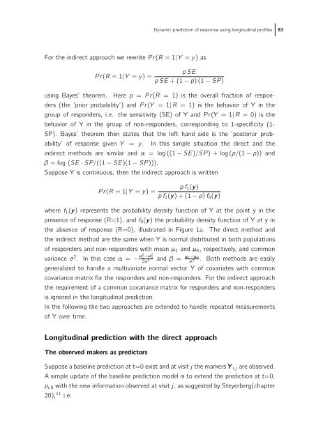
For the indirect approach we rewrite Pr(R =1| Y = y) as
Pr(R =1| Y = y) =
Dynamic prediction of response using longitudinal profi les 83
pSE
pSE+(1− p)(1− SP)
using Bayes’ theorem. Here p = Pr(R = 1) is the overall fraction of respon-
ders (the ’prior probability’) and Pr(Y =1| R = 1) is the behavior of Y in the
group of responders, i.e. the sensitivity (SE) of Y and Pr(Y =1| R =0)isthe
behavior of Y in the group of non-responders, corresponding to 1-specificity (1-
SP). Bayes’ theorem then states that the left hand side is the ’posterior probability’
of response given Y = y. In this simple situation the direct and the
indirect methods are similar and α = log ((1 − SE)/SP ) + log (p/(1 − p)) and
β = log (SE · SP/((1 − SE)(1 − SP))).
Suppose Y is continuous, then the indirect approach is written
Pr(R =1| Y = y) =
p f1(y)
p f1(y)+(1− p) f0(y)
where f1(y) represents the probability density function of Y at the point y in the
presence of response (R=1), and f0(y) the probability density function of Y at y in
the absence of response (R=0), illustrated in Figure 1a. The direct method and
the indirect method are the same when Y is normal distributed in both populations
of responders and non-responders with mean μ1 and μ0, respectively, and common
variance σ2 . In this case α = − μ2 1−μ2 0
2σ2 and β = μ1−μ0
σ2 . Both methods are easily
generalized to handle a multivariate normal vector Y of covariates with common
covariance matrix for the responders and non-responders. For the indirect approach
the requirement of a common covariance matrix for responders and non-responders
is ignored in the longitudinal prediction.
In the following the two approaches are extended to handle repeated measurements
of Y over time.
Longitudinal prediction with the direct approach
The observed makers as predictors
Suppose a baseline prediction at t=0 exist and at visit j the markers Y i,j are observed.
A simple update of the baseline prediction model is to extend the prediction at t=0,
pi,0 with the new information observed at visit j, as suggested by Steyerberg(chapter
20), 11 i.e.