View PDF Version - RePub - Erasmus Universiteit Rotterdam

Appendix
Discriminant analysis using a MLMM with a normal mixture 169
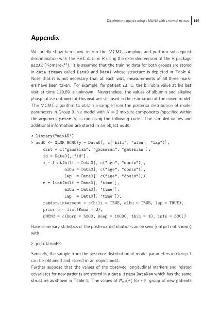
We briefly show here how to run the MCMC sampling and perform subsequent
discrimination with the PBC data in R using the extended version of the R package
mixAK (Komárek14 ). It is assumed that the training data for both groups are stored
in data.frames called Data0 and Data1 whose structure is depicted in Table 4.
Note that it is not necessary that at each visit, measurements of all three markers
have been taken. For example, for patient id=1, the bilirubin value at his last
visit at time 119.69 is unknown. Nevertheless, the values of albumin and alkaline
phosphatase obtained at this visit are still used in the estimation of the mixed model.
The MCMC algorithm to obtain a sample from the posterior distribution of model
parameters in Group 0 in a model with K = 2 mixture components (specified within
the argument prior.b) is run using the following code. The sampled values and
additional information are stored in an object mod0.
¿ library(”mixAK”)
¿ mod0 ¡- GLMM˙MCMC(y = Data0[, c(”bili”, ”albu”, ”lap”)],
dist = c(”gaussian”, ”gaussian”, ”gaussian”),
id = Data0[, ”id”],
x = list(bili = Data0[, c(”age”, ”dosis”)],
albu = Data0[, c(”age”, ”dosis”)],
lap = Data0[, c(”age”, ”dosis”)]),
z = list(bili = Data0[, ”time”],
albu = Data0[, ”time”],
lap = Data0[, ”time”]),
random.intercept = c(bili = TRUE, albu = TRUE, lap = TRUE),
prior.b = list(Kmax = 2),
nMCMC = c(burn = 5000, keep = 10000, thin = 10, info = 500))
Basic summary statistics of the posterior distribution can be seen (output not shown)
with
¿ print(mod0)
Similarly, the sample from the posterior distribution of model parameters in Group 1
can be obtained and stored in an object mod1.
Further suppose that the values of the observed longitudinal markers and related
covariates for new patients are stored in a data.frame DataNew which has the same
structure as shown in Table 4. The values of Pg,i(τ) fori∈ group of new patients