View PDF Version - RePub - Erasmus Universiteit Rotterdam

Dynamic prediction of response using longitudinal profi les 87
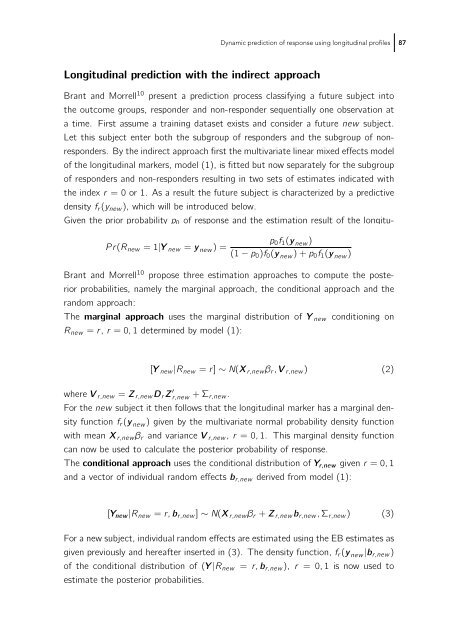
Longitudinal prediction with the indirect approach
Brant and Morrell 10 present a prediction process classifying a future subject into
the outcome groups, responder and non-responder sequentially one observation at
a time. First assume a training dataset exists and consider a future new subject.
Let this subject enter both the subgroup of responders and the subgroup of nonresponders.
By the indirect approach first the multivariate linear mixed effects model
of the longitudinal markers, model (1), is fitted but now separately for the subgroup
of responders and non-responders resulting in two sets of estimates indicated with
the index r = 0 or 1. As a result the future subject is characterized by a predictive
density fr (ynew), which will be introduced below.
Given the prior probability p0 of response and the estimation result of the longitu-
Pr(Rnew =1|Y new = y new) =
p0f1(y new)
(1 − p0)f0(y new)+p0f1(y new)
Brant and Morrell10 propose three estimation approaches to compute the posterior
probabilities, namely the marginal approach, the conditional approach and the
random approach:
The marginal approach uses the marginal distribution of Y new conditioning on
Rnew = r, r =0, 1 determined by model (1):
where V r,new = Zr,newDr Z ′ r,new +Σr,new.
[Y new|Rnew = r] ∼ N(Xr,newβr , V r,new) (2)
For the new subject it then follows that the longitudinal marker has a marginal den-
sity function fr (y new) given by the multivariate normal probability density function
with mean Xr,newβr and variance V r,new, r =0, 1. This marginal density function
can now be used to calculate the posterior probability of response.
The conditional approach uses the conditional distribution of Yr,new given r =0, 1
and a vector of individual random effects br,new derived from model (1):
[Ynew|Rnew = r,br,new] ∼ N(Xr,newβr + Zr,newbr,new, Σr,new) (3)
For a new subject, individual random effects are estimated using the EB estimates as
given previously and hereafter inserted in (3). The density function, fr (y new|br,new)
of the conditional distribution of (Y |Rnew = r,br,new), r =0, 1 is now used to
estimate the posterior probabilities.