View PDF Version - RePub - Erasmus Universiteit Rotterdam

Dynamic prediction of response using longitudinal profi les 93
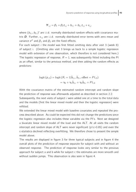
Y i,j = β1 + β2ti,j + b1,i + b2,iti,j + ɛi,j
where (b1,i,b2,i) ′ are i.i.d. normally distributed random effects with covariance ma-
trix D. Further, ɛi,j are i.i.d. normally distributed error terms with zero mean and
variance σ 2 and β1 and β2 are the fixed effects.
For each subject i the model was first fitted omitting data after visit 3 (week 8)
of subject i. (Omitting also visit 3 brings us back to a simple logistic regression
model with extension of one observation, which therefore is not considered here.)
The logistic regression of response, R = 1, was subsequently fitted including the PI
as an offset, similar to the previous method, and then adding the random effects as
predictors:
logit (pi,3) =logit (Ri =1|ˆb1,i, ˆb2,i, offset = PIi,0)
= γ0 + γ1 ˆb1,i + γ2 ˆb2,i + PIi,0
With the covariance matrix of the estimated random intercept and random slope
the prediction of response was afterwards adjusted as described in section 2.2.
Subsequently, the next visits of subject i were added one at a time to the total data
and the models (first the linear mixed model and then the logistic regression) were
refitted.
We extended the linear mixed model with baseline covariates and repeated the process
described above. As could be expected this did not change the predictions since
the logistic regression also includes these variables via the PI’s. Next we designed
a bivariate linear mixed model of the load and the ALT. At all visits the random
intercept and random slope of ALT were never significant (p’s>0.85) and even the
c-statistics declined reflecting overfitting. We therefore chose to present the simple
model above.
The results are displayed in figure 3 for three typical subjects and in figure 4 the
overall plots of the prediction of response separate for subject with and without an
observed response. The prediction of response looks very similar to the previous
approach for subject a and b while for subject c the estimates are more smooth and
without sudden jumps. This observation is also seen in figure 4.