- Page 1:
Statistical Models of Treatment Eff
- Page 4 and 5:
ISBN: 978-90-8559-069-9 © Bettina
- Page 6 and 7:
PROMOTIECOMMISSIE Promotor: Prof.dr
- Page 9 and 10:
CONTENTS Chapter 1. Introduction 11
- Page 13:
Cha pter 1 Introduction
- Page 16 and 17:
Chapter 1 14 Epidemiology Worldwide
- Page 18 and 19:
Chapter 1 16 Prediction models with
- Page 20 and 21:
Chapter 1 18 standard method fails
- Page 22 and 23:
Chapter 1 20 The extended non-linea
- Page 24 and 25:
Chapter 1 22 References 1. Blumberg
- Page 27:
Cha pter 2 Prediction of response t
- Page 30 and 31:
Chapter 2.1 28 ABSTRACT The aim of
- Page 32 and 33:
Chapter 2.1 30 been hepatitis B sur
- Page 34 and 35:
Chapter 2.1 32 HBV DNA decline The
- Page 36 and 37: Chapter 2.1 34 Figure 2 continued.
- Page 38 and 39: Chapter 2.1 36 Figure 4. Estimated
- Page 40 and 41: Chapter 2.1 38 DNA was observed in
- Page 42: Chapter 2.1 40 15. Kao JH. Role of
- Page 46 and 47: Chapter 2.2 44 ABSTRACT Background:
- Page 48 and 49: Chapter 2.2 46 low baseline HBV DNA
- Page 50 and 51: Chapter 2.2 48 patient subgroups wa
- Page 52 and 53: Chapter 2.2 50 p=0.002). Previous I
- Page 54 and 55: Chapter 2.2 52 Application of the m
- Page 56 and 57: Chapter 2.2 54 PEG-IFN, the proport
- Page 58 and 59: Chapter 2.2 56 References 1. Lavanc
- Page 60 and 61: Chapter 2.2 58 26. Bonino F, Lau GK
- Page 63 and 64: Chap ter 2.3 Prediction of the resp
- Page 65 and 66: INTRODUCTION Dynamic prediction of
- Page 67 and 68: Statistical analysis Dynamic predic
- Page 69 and 70: Dynamic prediction of response to P
- Page 71 and 72: Dynamic prediction of response to P
- Page 73 and 74: Dynamic prediction of response to P
- Page 75 and 76: Dynamic prediction of response to P
- Page 77 and 78: References Dynamic prediction of re
- Page 81 and 82: Cha pter 2.4 Dynamic prediction of
- Page 83 and 84: INTRODUCTION Dynamic prediction of
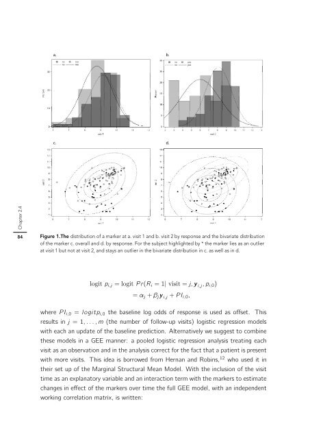
- Page 85: For the indirect approach we rewrit
- Page 89 and 90: Dynamic prediction of response usin
- Page 91 and 92: Dynamic prediction of response usin
- Page 93 and 94: Dynamic prediction of response usin
- Page 95 and 96: Dynamic prediction of response usin
- Page 97 and 98: Dynamic prediction of response usin
- Page 99 and 100: Dynamic prediction of response usin
- Page 101 and 102: Table 1. Results of different stopp
- Page 103 and 104: Dynamic prediction of response usin
- Page 105: Dynamic prediction of response usin
- Page 108 and 109: Chapter 2.5 106 ABSTRACT Peginterfe
- Page 110 and 111: Chapter 2.5 108 and placebo daily.
- Page 112 and 113: Chapter 2.5 110 for patients with a
- Page 114 and 115: Chapter 2.5 112 Mean HBV DNA declin
- Page 116 and 117: Chapter 2.5 114 peginterferon and n
- Page 118 and 119: Chapter 2.5 116 hepatocellular carc
- Page 120 and 121: Chapter 2.5 118 13. Werle-Lapostoll
- Page 122: Chapter 2.5 120 Greece - G Germanid
- Page 127 and 128: Chap ter 3.1 Long-term clinical out
- Page 129 and 130: INTRODUCTION Glycyrrhizin for IFN-n
- Page 131 and 132: Statistics Glycyrrhizin for IFN-non
- Page 133 and 134: Glycyrrhizin for IFN-non responders
- Page 135 and 136: Table 2. Time dependent Cox regress
- Page 137 and 138:
Glycyrrhizin for IFN-non responders
- Page 139 and 140:
Glycyrrhizin for IFN-non responders
- Page 143 and 144:
Cha pter 3.2 Discriminant analysis
- Page 145 and 146:
Introduction Discriminant analysis
- Page 147 and 148:
Discriminant analysis using a MLMM
- Page 149 and 150:
Estimation Discriminant analysis us
- Page 151 and 152:
Discriminant analysis using a MLMM
- Page 153 and 154:
where wi,k(y i, θ) = (k =1,...,K).
- Page 155 and 156:
Discriminant analysis using a MLMM
- Page 157 and 158:
Discriminant analysis using a MLMM
- Page 159 and 160:
Discriminant analysis using a MLMM
- Page 161 and 162:
Discriminant analysis using a MLMM
- Page 163 and 164:
Discriminant analysis using a MLMM
- Page 165 and 166:
Discriminant analysis using a MLMM
- Page 167 and 168:
Discriminant analysis using a MLMM
- Page 169 and 170:
Discriminant analysis using a MLMM
- Page 171 and 172:
Appendix Discriminant analysis usin
- Page 175:
Cha pter 4 Statistical models of ea
- Page 178 and 179:
Chapter 4.1 176 ABSTRACT Nucleoside
- Page 180 and 181:
Chapter 4.1 178 at day 1 at t =0 an
- Page 182 and 183:
Chapter 4.1 180 Table 1. Baseline c
- Page 184 and 185:
Chapter 4.1 182 Figure 1.
- Page 186 and 187:
Chapter 4.1 184 Figure 1. Viral dec
- Page 188 and 189:
Chapter 4.1 186 suppression in seru
- Page 190 and 191:
Chapter 4.1 188 13. Seifer M, Hamat
- Page 193 and 194:
Cha pter 4.2 Viral dynamics during
- Page 195 and 196:
INTRODUCTION Viral dynamics during
- Page 197 and 198:
Viral dynamics during tenofovir the
- Page 199 and 200:
Viral dynamics during tenofovir the
- Page 201 and 202:
log HBV DNA (copies/mL) 10.0 9.0 8.
- Page 203 and 204:
Viral dynamics during tenofovir the
- Page 205 and 206:
Viral dynamics during tenofovir the
- Page 207 and 208:
Viral dynamics during tenofovir the
- Page 211 and 212:
Chap ter 4.3 Modelling of early vir
- Page 213 and 214:
INTRODUCTION HBV viral kinetics dur
- Page 215 and 216:
HBV viral kinetics during PEG-IFN 2
- Page 217 and 218:
HBV viral kinetics during PEG-IFN 2
- Page 219 and 220:
HBV viral kinetics during PEG-IFN 2
- Page 221 and 222:
HBV viral kinetics during PEG-IFN 2
- Page 223 and 224:
HBV viral kinetics during PEG-IFN 2
- Page 225 and 226:
HBV viral kinetics during PEG-IFN 2
- Page 227 and 228:
HBV viral kinetics during PEG-IFN 2
- Page 229:
HBV viral kinetics during PEG-IFN 2
- Page 233 and 234:
SUMMARY AND CONCLUSION Summary and
- Page 235 and 236:
Summary and conclusion 233 The mode
- Page 237 and 238:
Summary and conclusion 235 The infe
- Page 239:
Summary and conclusion 237 Early st
- Page 243 and 244:
SAMENVATTING EN CONCLUSIE Samenvatt
- Page 245 and 246:
Samenvatting en conclusie 243 Er we
- Page 247 and 248:
Samenvatting en conclusie 245 Data
- Page 249 and 250:
Samenvatting en conclusie 247 Behan
- Page 253:
Dan kwoord
- Page 256 and 257:
Dankwoord 254 Lieve Marion en Margr
- Page 259 and 260:
BIBLI OGRAPHY Bibliography 257 1. K
- Page 261 and 262:
Bibliography 259 Interferon-ribavir
- Page 263 and 264:
Bibliography 261 Long term clinical
- Page 265 and 266:
Bibliography 263 Flares in chronic
- Page 267 and 268:
Bibliography 265 Genetic characteri
- Page 269:
Bibliography 267 106. Reijnders JG,