View PDF Version - RePub - Erasmus Universiteit Rotterdam

Chapter 2.4
88
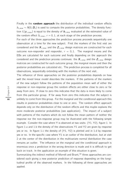
Finally in the random approach the distribution of the individual random effects
br,new ∼ N(0, Dr ) is used to compute the posterior probabilities. The density func-
tion fr (y r,new) is equal to the density of br,new evaluated at the estimated value of
the random effect ˆbr,new, r =0, 1, at each stage of the prediction process.
For each of the three approaches the prediction process proceeds sequentially one
observation at a time for the new subject. First the markers of the first visit are
considered and the Xr,new and the Zr,new design matrices are constructed for each
outcome non-responder and responder, r = 0, 1. The marginal means and the
EBs are calculated for each outcome and finally depending on the approach the
considered and the prediction process continues: the Xr,new and the Zr,new design
matrices are constructed for each outcome group, the marginal means and then the
posterior probabilities are calculated etc. The prediction process is completed for all
observations, sequentially extending with the markers of the next visit.
The influence of three approaches on the posterior probabilities depends on how
well the mixed linear model describes the markers. If the patterns of the markers
of the new subject follow the patterns of the population mean well of either the
response or non-response group the random effects are either close to zero or far
away from zero. If close to zero this indicates that the data is more likely to come
from this particular group. If far away from zero this indicates that the subject is
unlikely to come from this group. For the marginal and the conditional approach this
results in posterior probabilities close to one or zero. The random effect approach
depends only on the distribution of the random effects and this maybe explains the
more moderate posterior probabilities (see application). The impact of a subject
with patterns of the markers which do not follow the mean pattern of neither the
response nor the non-response group may be illustrated with the following simple
example. Consider the case where Y is observed at two visits: (Y1, Y2), figure 1. In
figure 1.a and 1.b the density of the observations Y1 and Y2 are given by response
yes or no. In figure 1.c the density of (Y1, Y2) is plotted and in 1.d by response
yes or no. In the specific case where Y1 is an outlier of the distribution, but at visit
2 at the center of the distribution in the multivariate normal distribution the case
remains an outlier. The influence on the marginal and the conditional approach is
enormous once a prediction in the wrong direction is made and it is difficult to get
back on track. In the application an example of this situation is given.
Summarizing the indirect method of Morrell and Brant, 10 three approaches are considered
each giving a new posterior prediction of response depending on the longitudinal
profile of the observed markers. In the following all three approaches are
applied.