View PDF Version - RePub - Erasmus Universiteit Rotterdam

Discriminant analysis using a MLMM with a normal mixture 161
Further, we explored the properties of the discrimination procedures based on Pg,i(τ)
from different models (K =1, 2) and different discrimination approaches (marginal,
conditional, random effects) in the following way. For each subject, each model
and discrimination approach, the evolution � �
P1,i(τ) :τ ≤ ti,ni was approximated
from computed values of P1,i(ti,1),...,P1,i(ti,n∗) as piecewise linear (as shown in
i
Figure 3). The values of P1,i(t), for t =0, 1,...,60 months, from patients whose
last visit happened at time t or later were subsequently used to draw receiver operating
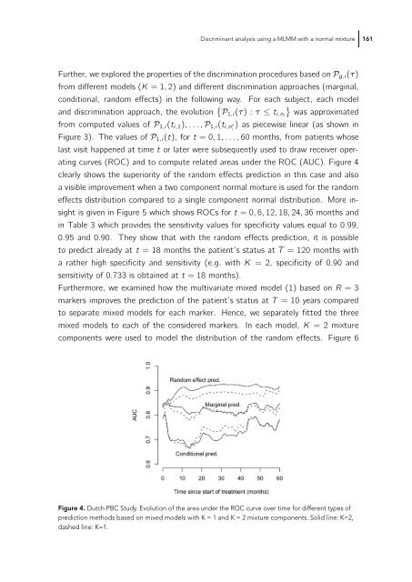
curves (ROC) and to compute related areas under the ROC (AUC). Figure 4
clearly shows the superiority of the random effects prediction in this case and also
a visible improvement when a two component normal mixture is used for the random
effects distribution compared to a single component normal distribution. More insight
is given in Figure 5 which shows ROCs for t =0, 6, 12, 18, 24, 36 months and
in Table 3 which provides the sensitivity values for specificity values equal to 0.99,
0.95 and 0.90. They show that with the random effects prediction, it is possible
to predict already at t = 18 months the patient’s status at T = 120 months with
a rather high specificity and sensitivity (e.g. with K = 2, specificity of 0.90 and
sensitivity of 0.733 is obtained at t = 18 months).
Furthermore, we examined how the multivariate mixed model (1) based on R =3
markers improves the prediction of the patient’s status at T = 10 years compared
to separate mixed models for each marker. Hence, we separately fitted the three
mixed models to each of the considered markers. In each model, K = 2 mixture
components were used to model the distribution of the random effects. Figure 6
Figure 4. Dutch PBC Study. Evolution of the area under the ROC curve over time for different types of
prediction methods based on mixed models with K = 1 and K = 2 mixture components. Solid line: K=2,
dashed line: K=1.