View PDF Version - RePub - Erasmus Universiteit Rotterdam

Chapter 2.4
86
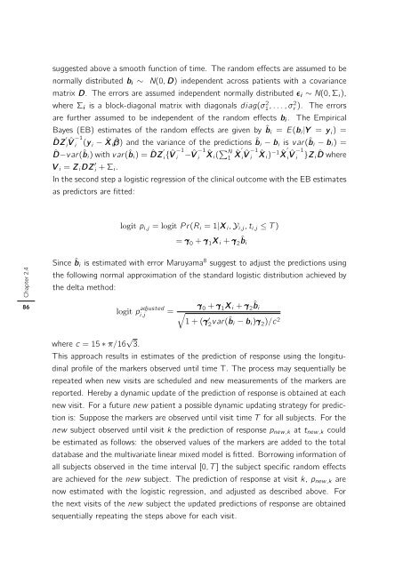
suggested above a smooth function of time. The random effects are assumed to be
normally distributed bi ∼ N(0, D) independent across patients with a covariance
matrix D. The errors are assumed independent normally distributed ɛi ∼ N(0, Σi),
where Σi is a block-diagonal matrix with diagonals diag(σ2 1 ,...,σ2 r ). The errors
are further assumed to be independent of the random effects bi . The Empirical
Bayes (EB) estimates of the random effects are given by ˆbi = E(bi|Y = y i)=
ˆDZ ′ −1
ˆV i i (y i − ˆXi ˆβ) and the variance of the predictions ˆbi − bi is var(ˆbi − bi) =
ˆD−var(ˆbi) with var(ˆbi) = ˆDZ ′
i{ˆV −1
i − ˆV −1
i ˆXi( � ′
N −1
ˆX ˆV 1 i i ˆXi) −1 ˆX ′ −1
ˆV i i }Zi ˆD where
V i = ZiDZ ′ i +Σi.
In the second step a logistic regression of the clinical outcome with the EB estimates
as predictors are fitted:
where c =15∗ π/16 √ 3.
logit pi,j = logit Pr(Ri =1|Xi, Yi,j,ti,j ≤ T )
logit p adjusted
i,j
= γ 0 + γ 1Xi + γ 2 ˆbi
Since ˆbi is estimated with error Maruyama8 suggest to adjust the predictions using
the following normal approximation of the standard logistic distribution achieved by
the delta method:
γ0 + γ1Xi + γ ˆbi 2
= �
1+(γ ′ 2var(ˆbi − bi)γ2)/c 2
This approach results in estimates of the prediction of response using the longitudinal
profile of the markers observed until time T. The process may sequentially be
repeated when new visits are scheduled and new measurements of the markers are
reported. Hereby a dynamic update of the prediction of response is obtained at each
new visit. For a future new patient a possible dynamic updating strategy for prediction
is: Suppose the markers are observed until visit time T for all subjects. For the
new subject observed until visit k the prediction of response pnew,k at tnew,k could
be estimated as follows: the observed values of the markers are added to the total
database and the multivariate linear mixed model is fitted. Borrowing information of
all subjects observed in the time interval [0,T] the subject specific random effects
are achieved for the new subject. The prediction of response at visit k, pnew,k are
now estimated with the logistic regression, and adjusted as described above. For
the next visits of the new subject the updated predictions of response are obtained
sequentially repeating the steps above for each visit.