- Page 1 and 2:
Exceptional Argentina Di Tella, Gla
- Page 3 and 4:
A third explanation of Argentina’
- Page 5 and 6:
Maddison's "Western Offshoots" by l
- Page 7 and 8:
A final point on this mechanistic a
- Page 9 and 10:
GDP in 1900 at 12,100 (in constant
- Page 11 and 12:
nationalized railways and banks, to
- Page 13 and 14:
country interacted with initial con
- Page 15 and 16:
1900. As there is an extremely stro
- Page 17 and 18:
Between the 1940s and 1970s income
- Page 19 and 20:
particularly in terms of food consu
- Page 21 and 22:
Even before the 2001 crisis, Argent
- Page 23 and 24:
Scandinavia and Northern Europe the
- Page 25 and 26:
Figure 4. A modified Human Developm
- Page 27 and 28:
Figure 6. Per capita GDP across Arg
- Page 29 and 30:
production 15 . Moreover, beyond st
- Page 31 and 32:
Figure 10. Average weight of export
- Page 33 and 34:
etween the prewar export-led growth
- Page 35 and 36:
which was wholly bound to local dem
- Page 37 and 38:
protectionism", certainly stronger
- Page 39 and 40:
agricultural pastures and cropland
- Page 41 and 42:
far. Argentina's differential popul
- Page 43 and 44:
Appendix Figure A. 1. Argentina's r
- Page 45 and 46:
Peru 35 38 25 34 34 34 32 29 26 27
- Page 47 and 48:
Like the Llach paper, the Campante
- Page 49 and 50:
I. Introduction Both Buenos Aires a
- Page 51 and 52:
across the ocean. Over the course o
- Page 53 and 54:
Buenos Aires’ hinterland rose dra
- Page 55 and 56:
significantly greater education lev
- Page 57 and 58:
Why is there such a difference in l
- Page 59 and 60:
illion dollars today). Each Chicago
- Page 61 and 62:
Chicago also appears to have been a
- Page 63 and 64:
casualties. Roca secured the presid
- Page 65 and 66:
capital to St. Petersburg he was pr
- Page 67 and 68:
and the logarithm of per capita GDP
- Page 69 and 70:
Moreover, years of schooling today
- Page 71 and 72:
y its overwhelming political import
- Page 73 and 74:
200 Figure 2a: Annual Wage Data 187
- Page 75 and 76:
Figure 3: Real Monthly Wages in Chi
- Page 77 and 78:
Log GDP per capita 2000 5 6 7 8 9 1
- Page 79 and 80:
Figure 7 Log GDP per capita 2000 7
- Page 81 and 82:
Table 2: Top 5 Industries in Chicag
- Page 83 and 84:
Table 4: 19th Century Variables and
- Page 85 and 86:
A simple calculation suggests that
- Page 87 and 88:
toy model with a minimum of paramet
- Page 89 and 90:
were lifted, but import taxes remai
- Page 91 and 92:
to compute that the MPK term above
- Page 93 and 94:
versus foreigners, on most occasion
- Page 95 and 96:
X institutions policies income p
- Page 97 and 98:
series variation. The coincidence o
- Page 99 and 100:
Figure 1—The Great Divergence and
- Page 101 and 102:
Figure 3—Trade taxes
- Page 103 and 104:
Transition Remarks The previous ess
- Page 105 and 106:
CHAPTER FOUR Argentine Trade Polici
- Page 107 and 108:
Argentine comparative advantage lie
- Page 109 and 110:
thousands of product lines in Argen
- Page 111 and 112:
Japan). Third, the agricultural pro
- Page 113 and 114:
different preferences over trade pr
- Page 115 and 116:
two nomenclatures had to be manuall
- Page 117 and 118:
esult, soybeans were finally adopte
- Page 119 and 120:
Figure 1 Trade Openness Exports + I
- Page 121 and 122:
Figure 5 Relative Sectoral Protecti
- Page 123 and 124:
Figure 7 Average Export Taxes 0 10
- Page 125 and 126:
Figure 9 Average Export Taxes at 2-
- Page 127 and 128:
Figure 11 Evolution of Argentine Ag
- Page 129 and 130:
Figure 13 Yields in Agriculture: Wh
- Page 131 and 132:
Table 2 Livestock per Capita 1895 C
- Page 133 and 134:
Table 5 Mean Share of Exports (Impo
- Page 135 and 136:
Table 7 Tariff Statistics for perio
- Page 137 and 138:
Table 9 Evolution of Industrial Pro
- Page 139 and 140:
CHAPTER FIVE Path-Dependent Import-
- Page 141 and 142:
actors, and they were demanding pro
- Page 143 and 144:
the primary sector, using land and
- Page 145 and 146:
Figure 1: The Long Run: Four Region
- Page 147 and 148:
Finally, in the reversal of pattern
- Page 149 and 150:
Figure 3: Medium Run Preferences ov
- Page 151 and 152:
sector to give rise to a protection
- Page 153 and 154:
technological improvements or incre
- Page 155 and 156:
Argentina did relatively well when
- Page 157 and 158:
World War, a second globalization e
- Page 159 and 160:
Argentine primary sector and ensure
- Page 161 and 162:
Clearly, world market conditions we
- Page 163 and 164:
for the years to come. The most imp
- Page 165 and 166:
governments zigzagged in their poli
- Page 167 and 168:
public spending on infrastructure s
- Page 169 and 170:
understand the rise of the urban-ru
- Page 171 and 172:
To sum up, by the beginning of the
- Page 173 and 174:
has a comparative advantage in the
- Page 175 and 176:
L λ = m L K κ = m K That is, λ i
- Page 177 and 178:
K c a = 1− α 1−α T A ( κ )
- Page 179 and 180:
Given a set of parameters ϒ , φ a
- Page 181 and 182:
consumption of good i. For any agen
- Page 183 and 184:
Proposition 3 In the short run, pro
- Page 185 and 186:
ρ 1/ 1 ρ ρ 1 ( ξ ξ ) 1 TT K ,
- Page 187 and 188:
Up to 2008, the FPV government had
- Page 189 and 190:
negative correlation between the pr
- Page 191 and 192:
policies would, supposedly, eviscer
- Page 193 and 194:
I. Introduction In a seminal study,
- Page 195 and 196:
terms, Peronist beliefs in the 1990
- Page 197 and 198:
Several authors have emphasized the
- Page 199 and 200:
foreign capital and trade as the gl
- Page 201 and 202:
of already available information. A
- Page 203 and 204:
having the need to do more than wak
- Page 205 and 206:
Argentines (who implement these pol
- Page 207 and 208:
opinion about elements of capitalis
- Page 209 and 210:
intense (the proportion is under 1.
- Page 211 and 212:
involved in social ordering that wi
- Page 213 and 214:
cost of the deviating firm, since w
- Page 215 and 216:
Admissible Region Bounds on w b Nex
- Page 217 and 218:
The previous proposition may be par
- Page 219 and 220:
and note that Peron insists on the
- Page 221 and 222:
Appendix 2: Definitions of Variable
- Page 223 and 224:
Table II: The Beliefs of Peronists
- Page 225 and 226:
Transition Remarks The previous cha
- Page 227 and 228:
CHAPTER SEVEN A Short Episodic Hist
- Page 229 and 230:
the income distribution between 193
- Page 231 and 232:
empirical evidence and on existing
- Page 233 and 234:
of commodities. The country was off
- Page 235 and 236:
accounts increased by 8% between 19
- Page 237 and 238:
Argentina in 1942 (4.1%) is not ver
- Page 239 and 240:
This change in inequality is also r
- Page 241 and 242:
1982, when Mexico’s default on it
- Page 243 and 244:
1995. While growth bounced back qui
- Page 245 and 246:
The main characteristics of this ep
- Page 247 and 248:
skilled workers that more than offs
- Page 249 and 250:
Household Expenditure Survey. An in
- Page 251 and 252:
The relationship between internatio
- Page 253 and 254:
machinery and equipment can acceler
- Page 255 and 256:
occurred not only in production tec
- Page 257 and 258:
a relative abundance of rents to sh
- Page 259 and 260:
even when the number of well-off in
- Page 261 and 262:
and similar patterns emerge when co
- Page 263 and 264:
This chapter described the level an
- Page 265 and 266:
Transition Remarks Economic success
- Page 267 and 268:
CHAPTER EIGHT Why do Argentines tru
- Page 269 and 270:
in the 1970s and 1980s. Despite the
- Page 271 and 272:
Figure 5. Percentage of the populat
- Page 273 and 274: analysis of the Argentinean and Chi
- Page 275 and 276: observationally equivalent individu
- Page 277 and 278: the low rank policeman. 13 4. The C
- Page 279 and 280: Figure 7. Share of people having a
- Page 281 and 282: 6. Why did the Argentinean Police d
- Page 283 and 284: instability, σ, a worried leader h
- Page 285 and 286: the deeper question of why the Arge
- Page 287 and 288: Table 2. Comparative facts for cano
- Page 289 and 290: of formal education, whereas in the
- Page 291 and 292: only bargaining tool to get money.
- Page 293 and 294: Table 6. Tierra del Fuego Subinspec
- Page 295 and 296: 4. Police deaths during the 20th ce
- Page 297 and 298: Of course, these conclusions depend
- Page 299 and 300: “stop go” dynamics 4 ). In fact
- Page 301 and 302: income distribution and earnings gr
- Page 303 and 304: Figure 2. Basic Statistics Food Clo
- Page 305 and 306: Table 2 Dep. Var.: Share of food Sm
- Page 307 and 308: Figure 3. Variety in food retailing
- Page 309 and 310: Table 3 Dep. Var.: Share of food at
- Page 311 and 312: 3.3 Income distribution effects The
- Page 313 and 314: Figure 6. Individual Effects Using
- Page 315 and 316: Expenditure Income 5000 6000 4000 4
- Page 317 and 318: Figure 10. Income distribution Dens
- Page 319 and 320: Appendix A: Estimation strategy Est
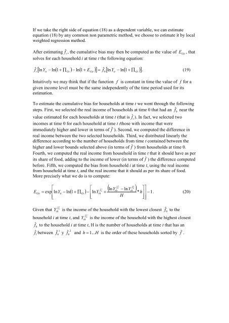
- Page 321 and 322: w ijt where [ ln( 1+ ∏ ) − ln(
- Page 323: 2.2 Income distribution effects Fol
- Page 327 and 328: Appendix C: Additional tables C1: B
- Page 329 and 330: C3: Table 3 coefficients Dummy for
- Page 331 and 332: CONCLUSION 20 th century Argentina
- Page 333 and 334: can be harbingers of worse things t
- Page 335 and 336: Ahumada, Hildegart, Alfredo Canaves
- Page 337 and 338: Barro, Robert J. 2005. “Rare Even
- Page 339 and 340: Burzaco, Eugenio et al. 2004. “Ma
- Page 341 and 342: Cortés Conde, Roberto and María M
- Page 343 and 344: Di Tella, Rafael, Juan Dubra and Ro
- Page 345 and 346: Gaggero, Horacio and Alicia Garro.
- Page 347 and 348: Gerchunoff, Pablo, Fernando Rocchi
- Page 349 and 350: James, Daniel. 1988. “October 17
- Page 351 and 352: Maddison, Angus. 2006. The World Ec
- Page 353 and 354: Piketty, T. 2003. “Income Inequal
- Page 355 and 356: Spiller, Pablo and Mariano Tommasi.
- Page 357: Williamson, Jeffrey G. 1995. “The


