Exceptional Argentina Di Tella, Glaeser and Llach - Thomas Piketty

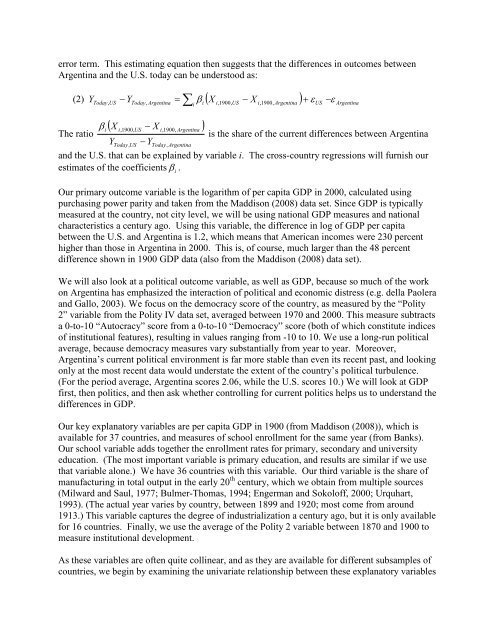
error term. This estimating equation then suggests that the differences in outcomes between
Argentina and the U.S. today can be understood as:
(2) YToday,
US
− YToday,
Argentina
= ∑ β ( )
i i
X
i,1900,
US
− X
i,1900,
Argentina
+ ε
US
−ε
Argentina
β ( X − X )
i
i,1900,
US
i,1900,
Argentina
The ratio
is the share of the current differences between Argentina
YToday,
US
− YToday,
Argentina
and the U.S. that can be explained by variable i. The cross-country regressions will furnish our
estimates of the coefficients β .
i
Our primary outcome variable is the logarithm of per capita GDP in 2000, calculated using
purchasing power parity and taken from the Maddison (2008) data set. Since GDP is typically
measured at the country, not city level, we will be using national GDP measures and national
characteristics a century ago. Using this variable, the difference in log of GDP per capita
between the U.S. and Argentina is 1.2, which means that American incomes were 230 percent
higher than those in Argentina in 2000. This is, of course, much larger than the 48 percent
difference shown in 1900 GDP data (also from the Maddison (2008) data set).
We will also look at a political outcome variable, as well as GDP, because so much of the work
on Argentina has emphasized the interaction of political and economic distress (e.g. della Paolera
and Gallo, 2003). We focus on the democracy score of the country, as measured by the “Polity
2” variable from the Polity IV data set, averaged between 1970 and 2000. This measure subtracts
a 0-to-10 “Autocracy” score from a 0-to-10 “Democracy” score (both of which constitute indices
of institutional features), resulting in values ranging from -10 to 10. We use a long-run political
average, because democracy measures vary substantially from year to year. Moreover,
Argentina’s current political environment is far more stable than even its recent past, and looking
only at the most recent data would understate the extent of the country’s political turbulence.
(For the period average, Argentina scores 2.06, while the U.S. scores 10.) We will look at GDP
first, then politics, and then ask whether controlling for current politics helps us to understand the
differences in GDP.
Our key explanatory variables are per capita GDP in 1900 (from Maddison (2008)), which is
available for 37 countries, and measures of school enrollment for the same year (from Banks).
Our school variable adds together the enrollment rates for primary, secondary and university
education. (The most important variable is primary education, and results are similar if we use
that variable alone.) We have 36 countries with this variable. Our third variable is the share of
manufacturing in total output in the early 20 th century, which we obtain from multiple sources
(Milward and Saul, 1977; Bulmer-Thomas, 1994; Engerman and Sokoloff, 2000; Urquhart,
1993). (The actual year varies by country, between 1899 and 1920; most come from around
1913.) This variable captures the degree of industrialization a century ago, but it is only available
for 16 countries. Finally, we use the average of the Polity 2 variable between 1870 and 1900 to
measure institutional development.
As these variables are often quite collinear, and as they are available for different subsamples of
countries, we begin by examining the univariate relationship between these explanatory variables