PENELOPE 2003 - OECD Nuclear Energy Agency

4.1. Elastic scattering 131
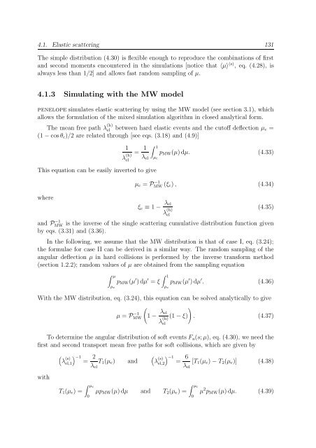
The simple distribution (4.30) is flexible enough to reproduce the combinations of first
and second moments encountered in the simulations [notice that 〈µ〉 (s) , eq. (4.28), is
always less than 1/2] and allows fast random sampling of µ.
4.1.3 Simulating with the MW model
penelope simulates elastic scattering by using the MW model (see section 3.1), which
allows the formulation of the mixed simulation algorithm in closed analytical form.
The mean free path λ (h)
el between hard elastic events and the cutoff deflection µ c =
(1 − cos θ c )/2 are related through [see eqs. (3.18) and (4.9)]
1
λ (h)
el
This equation can be easily inverted to give
where
= 1
λ el
∫ 1
µ c
p MW (µ) dµ. (4.33)
µ c = P −1
MW (ξ c ) , (4.34)
ξ c ≡ 1 − λ el
λ (h)
el
(4.35)
and P −1
MW is the inverse of the single scattering cumulative distribution function given
by eqs. (3.31) and (3.36).
In the following, we assume that the MW distribution is that of case I, eq. (3.24);
the formulae for case II can be derived in a similar way. The random sampling of the
angular deflection µ in hard collisions is performed by the inverse transform method
(section 1.2.2); random values of µ are obtained from the sampling equation
∫ µ
µ c
p MW (µ ′ ) dµ ′ = ξ
∫ 1
µ c
p MW (µ ′ ) dµ ′ . (4.36)
With the MW distribution, eq. (3.24), this equation can be solved analytically to give
µ = P −1
MW
(
1 − λ )
el
(1 − ξ) . (4.37)
To determine the angular distribution of soft events F a (s; µ), eq. (4.30), we need the
first and second transport mean free paths for soft collisions, which are given by
λ (h)
el
with
( )
(s) −1 2
λ el,1 = T 1 (µ c )
λ el
and
( )
(s) −1 6
λ el,2 = [T 1 (µ c ) − T 2 (µ c )] (4.38)
λ el
T 1 (µ c ) =
∫ µc
0
µp MW (µ) dµ and T 2 (µ c ) =
∫ µc
0
µ 2 p MW (µ) dµ. (4.39)