Segmentation of 3D Tubular Tree Structures in Medical Images ...

24 Chapter 2. Extraction of Tubular Structures
(a) Original (b) σ = 1.0 (c) σ = 2.5 (d) σ = 5.0 (e) σ = 10.0
(f) Original (g) σ = 1.0 (h) σ = 2.5 (i) σ = 5.0 (j) σ = 10.0
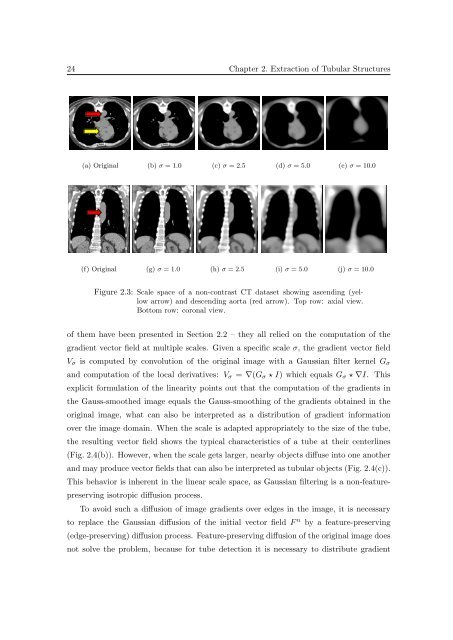
Figure 2.3: Scale space of a non-contrast CT dataset showing ascending (yellow
arrow) and descending aorta (red arrow). Top row: axial view.
Bottom row: coronal view.
of them have been presented in Section 2.2 – they all relied on the computation of the
gradient vector field at multiple scales. Given a specific scale σ, the gradient vector field
V σ is computed by convolution of the original image with a Gaussian filter kernel G σ
and computation of the local derivatives: V σ = ∇(G σ ⋆ I) which equals G σ ⋆ ∇I. This
explicit formulation of the linearity points out that the computation of the gradients in
the Gauss-smoothed image equals the Gauss-smoothing of the gradients obtained in the
original image, what can also be interpreted as a distribution of gradient information
over the image domain. When the scale is adapted appropriately to the size of the tube,
the resulting vector field shows the typical characteristics of a tube at their centerlines
(Fig. 2.4(b)). However, when the scale gets larger, nearby objects diffuse into one another
and may produce vector fields that can also be interpreted as tubular objects (Fig. 2.4(c)).
This behavior is inherent in the linear scale space, as Gaussian filtering is a non-featurepreserving
isotropic diffusion process.
To avoid such a diffusion of image gradients over edges in the image, it is necessary
to replace the Gaussian diffusion of the initial vector field F n by a feature-preserving
(edge-preserving) diffusion process. Feature-preserving diffusion of the original image does
not solve the problem, because for tube detection it is necessary to distribute gradient