Segmentation of 3D Tubular Tree Structures in Medical Images ...
Segmentation of 3D Tubular Tree Structures in Medical Images ...
Segmentation of 3D Tubular Tree Structures in Medical Images ...

You also want an ePaper? Increase the reach of your titles
YUMPU automatically turns print PDFs into web optimized ePapers that Google loves.
62 Chapter 3. Group<strong>in</strong>g and L<strong>in</strong>kage <strong>in</strong>to Connected Networks<br />
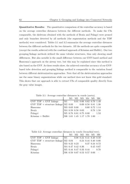
Quantitative Results: The quantitative comparison <strong>of</strong> the centerl<strong>in</strong>e accuracy is based<br />
on the average centerl<strong>in</strong>e distances between the different methods. To make the CSs<br />
comparable, the skeletons obta<strong>in</strong>ed with the methods <strong>of</strong> Bouix and Palagyi were pruned<br />
and only branches detected by all methods (the segmentation methods and the TDF<br />
methods) were considered. Tables 3.1 and 3.2 summarize the average centerl<strong>in</strong>e distances<br />
between the different methods for the two datasets. All the methods are quite comparable<br />
(except the results achieved with the comb<strong>in</strong>ed approach <strong>of</strong> Krissian and Bullitt). Our two<br />
group<strong>in</strong>g/l<strong>in</strong>kage methods utilized the same tubular structures, thus only show<strong>in</strong>g small<br />
differences. But also notable is the small difference between our GVF-based method and<br />
Hassouna’s approach on the airway tree, but this may be expla<strong>in</strong>ed s<strong>in</strong>ce this method is<br />
also based on the GVF. As these results show, the achieved centerl<strong>in</strong>e accuracy <strong>of</strong> our GVFbased<br />
tube detection and group<strong>in</strong>g/l<strong>in</strong>kage method is comparable to the variation found<br />
between different skeletonization approaches. Note that all the skeletonization approaches<br />
use the same b<strong>in</strong>ary segmentations while our method does not know this gold standard.<br />
This shows that our approach is able to extract CSs <strong>of</strong> comparable quality directly from<br />
the gray value images.<br />
Table 3.1: Average centerl<strong>in</strong>e distances <strong>in</strong> voxels (aorta).<br />
M1 M2 M3 M4 M5 M6<br />
GVF TDF + GVF l<strong>in</strong>kage M1 – 0.01 0.66 0.62 0.79 1.49<br />
GVF TDF + structure l<strong>in</strong>kage M2 0.03 – 0.69 0.58 0.81 1.38<br />
Hassouna M3 0.63 0.68 – 0.60 0.72 1.14<br />
Bouix M4 0.59 0.58 0.63 – 0.78 1.58<br />
Palagyi M5 0.78 0.81 0.75 0.80 – 1.53<br />
Krissian + Bullitt M6 1.61 1.45 1.17 1.70 1.60 –<br />
Table 3.2: Average centerl<strong>in</strong>e distances <strong>in</strong> voxels (bronchial tree).<br />
M1 M2 M3 M4 M5 M6<br />
GVF TDF + GVF l<strong>in</strong>kage M1 – 0.08 0.24 0.41 0.40 0.58<br />
GVF TDF + structure l<strong>in</strong>kage M2 0.04 – 0.24 0.44 0.40 0.66<br />
Hassouna M3 0.22 0.23 – 0.37 0.34 0.72<br />
Bouix M4 0.47 0.42 0.36 – 0.45 0.67<br />
Palagyi M5 0.44 0.47 0.33 0.44 – 0.70<br />
Krissian M6 0.59 0.67 0.53 0.57 0.66 –