Segmentation of 3D Tubular Tree Structures in Medical Images ...
Segmentation of 3D Tubular Tree Structures in Medical Images ...
Segmentation of 3D Tubular Tree Structures in Medical Images ...

Create successful ePaper yourself
Turn your PDF publications into a flip-book with our unique Google optimized e-Paper software.
2.5. Experiments 35<br />
However, the approach <strong>of</strong> Krissian does not produce any response between these closely<br />
tangent<strong>in</strong>g tubular objects <strong>in</strong> Fig. 2.7(e), <strong>in</strong> contrast to the example <strong>in</strong> Fig. 2.6(d) where<br />
it did.<br />
This behavior deserves a closer <strong>in</strong>vestigation and explanation. With Pock’s approach<br />
two different scale spaces are utilized where the scale at which the boundary <strong>in</strong>formation<br />
is obta<strong>in</strong>ed depends on a parameter η. Moreover, the relation between the radius <strong>of</strong> the<br />
tubular objects and the boundary <strong>in</strong>formation is non-l<strong>in</strong>ear (σ P 2 = r η with 0.0 ≤ η ≤ 1.0<br />
as expla<strong>in</strong>ed <strong>in</strong> Section 2.2.2), mean<strong>in</strong>g that the response also depends on the size <strong>of</strong> the<br />
tubular objects expla<strong>in</strong><strong>in</strong>g the different results between the two figures. The approach <strong>of</strong><br />
Pock addresses the problem <strong>of</strong> the pure Gaussian scale space methods (Frangi, Krissian),<br />
by comput<strong>in</strong>g the boundary <strong>in</strong>formation on a smaller scale. However, this computation<br />
<strong>of</strong> the boundary <strong>in</strong>formation on a smaller scale represents a trade<strong>of</strong>f with this method<br />
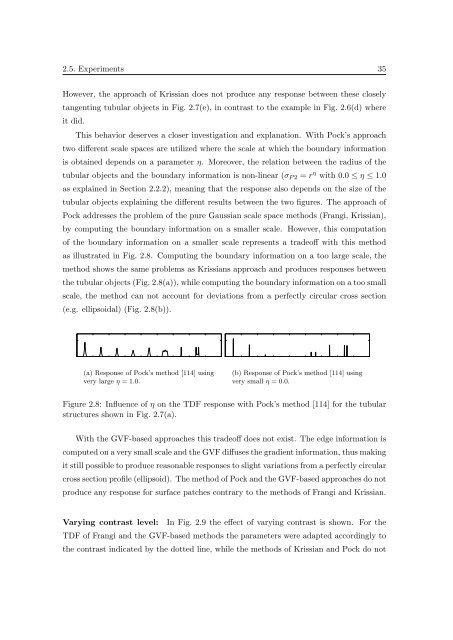
as illustrated <strong>in</strong> Fig. 2.8. Comput<strong>in</strong>g the boundary <strong>in</strong>formation on a too large scale, the<br />
method shows the same problems as Krissians approach and produces responses between<br />
the tubular objects (Fig. 2.8(a)), while comput<strong>in</strong>g the boundary <strong>in</strong>formation on a too small<br />
scale, the method can not account for deviations from a perfectly circular cross section<br />
(e.g. ellipsoidal) (Fig. 2.8(b)).<br />
50<br />
50<br />
0<br />
0<br />
0 200 400 600 800 1000 1200 1400 1600 18000 200 400 600 800 1000 1200 1400 1600 1800<br />
(a) Response <strong>of</strong> Pock’s method [114] us<strong>in</strong>g<br />
very large η = 1.0.<br />
(b) Response <strong>of</strong> Pock’s method [114] us<strong>in</strong>g<br />
very small η = 0.0.<br />
Figure 2.8: Influence <strong>of</strong> η on the TDF response with Pock’s method [114] for the tubular<br />
structures shown <strong>in</strong> Fig. 2.7(a).<br />
With the GVF-based approaches this trade<strong>of</strong>f does not exist. The edge <strong>in</strong>formation is<br />
computed on a very small scale and the GVF diffuses the gradient <strong>in</strong>formation, thus mak<strong>in</strong>g<br />
it still possible to produce reasonable responses to slight variations from a perfectly circular<br />
cross section pr<strong>of</strong>ile (ellipsoid). The method <strong>of</strong> Pock and the GVF-based approaches do not<br />
produce any response for surface patches contrary to the methods <strong>of</strong> Frangi and Krissian.<br />
Vary<strong>in</strong>g contrast level: In Fig. 2.9 the effect <strong>of</strong> vary<strong>in</strong>g contrast is shown. For the<br />
TDF <strong>of</strong> Frangi and the GVF-based methods the parameters were adapted accord<strong>in</strong>gly to<br />
the contrast <strong>in</strong>dicated by the dotted l<strong>in</strong>e, while the methods <strong>of</strong> Krissian and Pock do not