Vegetation Classification and Mapping Project Report - USGS

3 Base Map Class Development
3.1 Methods
3.1.1 Overview
To create the base map classes, the
mapping team, consisting primarily of
Monica McTeague (NAU) and Anne
Cully (NPS), developed GIS polygons
and labeled them to the finest floristic
level possible using a traditional
photointerpretation approach. The
resulting base map polygons are the finest
spatial data in the GIS database. Ideally,
each polygon represents a map class
that consists of one plant community
that is an association, alliance, or park
special; or one land-use class. However,
one-to-one correspondence of map
class to a single plant community is
sometimes not possible because mixed
or indistinguishable photosignatures on
the aerial photography make it diffcult
for the photointerpreter to distinguish
every plant community. In such cases, the
map class assigned represents a group of
associations, alliances, or park specials.
The group, management, and macrogroup
map classes described in Section 4 derive
from the base map classes.
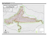
3.1.2 Imagery
The SCPN acquired new stereo aerial
photography of PEFO through the U.S.
Department of Agriculture’s Aerial
Photography Field Offce (APFO). APFO
subcontractor Photo Flight Geomatics,
of Tucson, Arizona, acquired the imagery
on September 13, 14, 17, and 19 of 2003;
an additional flight was made on June 17,
2004 to cover areas that were missed in
2003. The imagery was taken in true color
film at a scale of 1:6,000, with 20–40%
sidelap and 50–60% overlap. The APFO
provided two sets of 9 × 9-in contact prints
to the SCPN. The NAU and NPS mapping
team used the images for reference during
polygon delineation and labeling. Upon
project completion, one set of contact
prints will reside at PEFO and one at the
SCPN. Figures 6 and 7 show the flight lines
and photo centers.
3.1.3 Field Reconnaissance
The photointerpreters, Cully and
McTeague, conducted field reconnaissance
of plant communities and their
corresponding photosignatures during
March and October 2004; May, July,
August, October, and November 2005; and
April 2006, prior to and simultaneous to
delineating and labeling polygons. Cully
and McTeague traveled together in the
park for the first visits to ensure that they
had a consistent understanding of the flora
and plant communities. After the initial
visits, they divided the park into northern
and southern portions, and each took one
portion for photointerpretation.
Cully and McTeague visited 113 sites in
areas represented by photosignatures
that were not easily identifiable on
the aerial photography, and in areas
that were representative of vegetation
associations (fig. 8). At each site they
recorded (1) the geographic coordinates
of the site, (2) the vegetation structure
and composition (including dominant
species cover estimates), and (3) a brief
description of the site’s environmental
characteristics. They took two or more
digital photographs at each observation
point. For many sites, they recorded
additional field observations directly onto
transparent polyester sheets overlain
on the aerial photos (see section 3.1.4).
These were used in the lab as a guide
during photointerpretation. The data were
entered into a Microsoft® Access database
and each observation site was assigned a
provisional plant community assignment.
3.1.4 Base Map Class Polygons and
Labels
The NAU and NPS mapping team
delineated map polygons on a transparent
polyester sheet overlain on the true-color
aerial photographs. Adjoining photos
were used to determine the central area
on a particular photo frame with the least
distortion, known as the ‘effective area’;
this area was boxed in on the polyester
23