PERCOLATION AND DISORDERED SYSTEMS Geoffrey GRIMMETT
PERCOLATION AND DISORDERED SYSTEMS Geoffrey GRIMMETT
PERCOLATION AND DISORDERED SYSTEMS Geoffrey GRIMMETT

You also want an ePaper? Increase the reach of your titles
YUMPU automatically turns print PDFs into web optimized ePapers that Google loves.
11.1. Random Fractals<br />
Percolation and Disordered Systems 251<br />
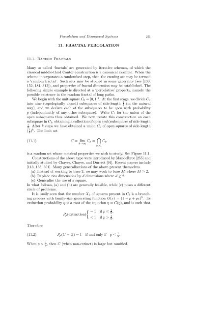
11. FRACTAL <strong>PERCOLATION</strong><br />
Many so called ‘fractals’ are generated by iterative schemes, of which the<br />
classical middle-third Cantor construction is a canonical example. When the<br />
scheme incorporates a randomised step, then the ensuing set may be termed<br />
a ‘random fractal’. Such sets may be studied in some generality (see [130,<br />
152, 184, 312]), and properties of fractal dimension may be established. The<br />
following simple example is directed at a ‘percolative’ property, namely the<br />
possible existence in the random fractal of long paths.<br />
We begin with the unit square C0 = [0, 1] 2 . At the first stage, we divide C0<br />
into nine (topologically closed) subsquares of side-length 1<br />
3 (in the natural<br />
way), and we declare each of the subsquares to be open with probability<br />
p (independently of any other subsquare). Write C1 for the union of the<br />
open subsquares thus obtained. We now iterate this construction on each<br />
subsquare in C1, obtaining a collection of open (sub)subsquares of side-length<br />
1<br />
9 . After k steps we have obtained a union Ck of open squares of side-length<br />
( 1<br />
3 )k . The limit set<br />
(11.1) C = lim<br />
k→∞ Ck = �<br />
is a random set whose metrical properties we wish to study. See Figure 11.1.<br />
Constructions of the above type were introduced by Mandelbrot [255] and<br />
initially studied by Chayes, Chayes, and Durrett [91]. Recent papers include<br />
[113, 133, 301]. Many generalisations of the above present themselves.<br />
(a) Instead of working to base 3, we may work to base M where M ≥ 2.<br />
(b) Replace two dimensions by d dimensions where d ≥ 2.<br />
(c) Generalise the use of a square.<br />
In what follows, (a) and (b) are generally feasible, while (c) poses a different<br />
circle of problems.<br />
It is easily seen that the number Xk of squares present in Ck is a branching<br />
process with family-size generating function G(x) = (1 − p + px) 9 . Its<br />
extinction probability η is a root of the equation η = G(η), and is such that<br />
Therefore<br />
k≥1<br />
Ck<br />
� 1 = 1 if p ≤ 9<br />
Pp(extinction)<br />
,<br />
< 1 if p > 1<br />
9 .<br />
(11.2) Pp(C = ∅) = 1 if and only if p ≤ 1<br />
9 .<br />
When p > 1<br />
9 , then C (when non-extinct) is large but ramified.