PERCOLATION AND DISORDERED SYSTEMS Geoffrey GRIMMETT
PERCOLATION AND DISORDERED SYSTEMS Geoffrey GRIMMETT
PERCOLATION AND DISORDERED SYSTEMS Geoffrey GRIMMETT

You also want an ePaper? Increase the reach of your titles
YUMPU automatically turns print PDFs into web optimized ePapers that Google loves.
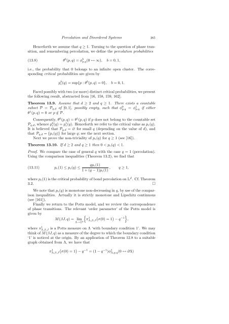
Percolation and Disordered Systems 265<br />
Henceforth we assume that q ≥ 1. Turning to the question of phase transition,<br />
and remembering percolation, we define the percolation probabilities<br />
(13.8) θ b (p, q) = φ b p,q(0 ↔ ∞), b = 0, 1,<br />
i.e., the probability that 0 belongs to an infinite open cluster. The corresponding<br />
critical probabilities are given by<br />
p b c (q) = sup{p : θb (p, q) = 0}, b = 0, 1.<br />
Faced possibly with two (or more) distinct critical probabilities, we present<br />
the following result, abstracted from [16, 158, 159, 162].<br />
Theorem 13.9. Assume that d ≥ 2 and q ≥ 1. There exists a countable<br />
subset P = Pq,d of [0, 1], possibly empty, such that φ 0 p,q = φ 1 p,q if either<br />
θ 1 (p, q) = 0 or p /∈ P.<br />
Consequently, θ0 (p, q) = θ1 (p, q) if p does not belong to the countable set<br />
Pq,d, whence p0 c (q) = p1c (q). Henceforth we refer to the critical value as pc(q).<br />
It is believed that Pq,d = ∅ for small q (depending on the value of d), and<br />
that Pq,d = {pc(q)} for large q; see the next section.<br />
Next we prove the non-triviality of pc(q) for q ≥ 1 (see [16]).<br />
Theorem 13.10. If d ≥ 2 and q ≥ 1 then 0 < pc(q) < 1.<br />
Proof. We compare the case of general q with the case q = 1 (percolation).<br />
Using the comparison inequalities (Theorem 13.2), we find that<br />
(13.11) pc(1) ≤ pc(q) ≤<br />
qpc(1)<br />
, q ≥ 1,<br />
1 + (q − 1)pc(1)<br />
where pc(1) is the critical probability of bond percolation on L d . Cf. Theorem<br />
3.2. �<br />
We note that pc(q) is monotone non-decreasing in q, by use of the comparison<br />
inequalities. Actually it is strictly monotone and Lipschitz continuous<br />
(see [161]).<br />
Finally we return to the Potts model, and we review the correspondence<br />
of phase transitions. The relevant ‘order parameter’ of the Potts model is<br />
given by<br />
M(βJ, q) = lim<br />
Λ→Zd �<br />
π 1 � � −1<br />
Λ,β,J σ(0) = 1 − q �<br />
,<br />
where π1 Λ,β,J is a Potts measure on Λ ‘with boundary condition 1’. We may<br />
think of M(βJ, q) as a measure of the degree to which the boundary condition<br />
‘1’ is noticed at the origin. By an application of Theorem 12.8 to a suitable<br />
graph obtained from Λ, we have that<br />
π 1 � � −1 −1 1<br />
Λ,β,J σ(0) = 1 − q = (1 − q )φΛ,p,q (0 ↔ ∂Λ)