PERCOLATION AND DISORDERED SYSTEMS Geoffrey GRIMMETT

260 Geoffrey Grimmett
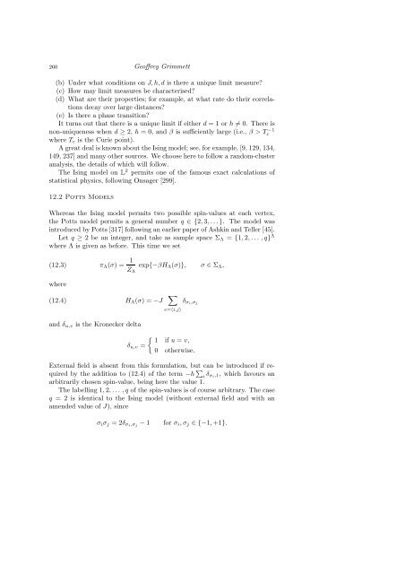
(b) Under what conditions on J, h, d is there a unique limit measure?
(c) How may limit measures be characterised?
(d) What are their properties; for example, at what rate do their correlations
decay over large distances?
(e) Is there a phase transition?
It turns out that there is a unique limit if either d = 1 or h �= 0. There is
non-uniqueness when d ≥ 2, h = 0, and β is sufficiently large (i.e., β > T −1
c
where Tc is the Curie point).
A great deal is known about the Ising model; see, for example, [9, 129, 134,
149, 237] and many other sources. We choose here to follow a random-cluster
analysis, the details of which will follow.
The Ising model on L2 permits one of the famous exact calculations of
statistical physics, following Onsager [299].
12.2 Potts Models
Whereas the Ising model permits two possible spin-values at each vertex,
the Potts model permits a general number q ∈ {2, 3, . . . }. The model was
introduced by Potts [317] following an earlier paper of Ashkin and Teller [45].
Let q ≥ 2 be an integer, and take as sample space ΣΛ = {1, 2, . . . , q} Λ
where Λ is given as before. This time we set
(12.3) πΛ(σ) = 1
where
ZΛ
(12.4) HΛ(σ) = −J �
and δu,v is the Kronecker delta
exp{−βHΛ(σ)}, σ ∈ ΣΛ,
e=〈i,j〉
δσi,σj
�
1 if u = v,
δu,v =
0 otherwise.
External field is absent from this formulation, but can be introduced if required
by the addition to (12.4) of the term −h �
i δσi,1, which favours an
arbitrarily chosen spin-value, being here the value 1.
The labelling 1, 2, . . . , q of the spin-values is of course arbitrary. The case
q = 2 is identical to the Ising model (without external field and with an
amended value of J), since
σiσj = 2δσi,σj − 1 for σi, σj ∈ {−1, +1}.