McKay, Donald. "Front matter" Multimedia Environmental Models ...

More documents

Recommendations

Info

QWASI Multi-segment Equations I(i) is total input (mol/h) to each reach from emissions, the atmosphere, and any tributaries. It does not include advective inputs from other reaches. DT(i) is the sum of D values for losses by reaction, burial, and volatilization plus all advective losses from water, including net loss to sediment. The (i) refers to reach 1, 2, 3, or 4. D(i,j) is water and particle flow between reaches i and j. J(i) is a D value for the net output from each reach. J(1) = DT(1) J(2) = DT(2) – D(2,1) D(1,2)/J(1) J(3) = DT(3) – D(3,2) D(2,3)/J(2) J(4) = DT(4) – D(4,3) D(3,4)/J(3) X(i) is the ratio of D values and is the fraction of the chemical in water and particle flow that enters downstream reach (reach 1 is upstream of reaches 2, 3, and 4). X(1) = D(1,2)/J(1) X(2) = D(2,3)/J(2) X(3) = D(3,4)/J(3) Fraction of total input received by each reach, including upstream reaches. Q(1) = I(1) Q(2) = I(2) + I(1) X(1) = I(2) + Q(1) X(1) Q(3) = I(3) + I(2) X(2) + I(1) X(1) X(2) = I(3) + Q(2) X(2) Q(4) = I(4) + I(3) X(3) + I(2) X(2) X(3) + I(1) X(1) X(2) X(3) = I(4) + Q(3) X(3) The solution for water fugacities fW(i) for each reach is as follows: fW(4) = {Q(4) + [fW(5) D(5,4)]}/J(4) fW(3) = {Q(3) + [fW(4) D(4,3)]}/J(3) fW(2) = {Q(4) + [fW(3) D(3,2)]}/J(2) fW(1) = {Q(4) + [fW(2) D(2,1)]}/J(1) The sediment fugacities fS(i) can then be calculated from the steady-state equation in Fig. 8.5. fs(i) = fw(i)(DD(i) + DT(i))/(DB(i) + DS(i) + DR(i) + DT(i)) with D values specific to each segment. Figure 8.8 Steady-state mass balance equations for a series of four QWASI models with flows in both directions. X, is a ratio of D values, namely the ratio of the box-to-box advective transfer D value and the total loss D value from the source. The denominators, J, contain terms for losses from each box, again modified by fractions undergoing box-to-box transfer. Inspection of the equations reveals the significance of each term. When the connections are more complex with branching, the equations must be modified ©2001 CRC Press LLC
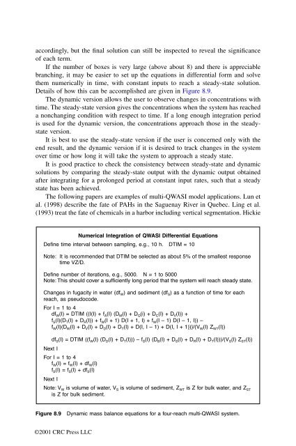
accordingly, but the final solution can still be inspected to reveal the significance of each term. If the number of boxes is very large (above about 8) and there is appreciable branching, it may be easier to set up the equations in differential form and solve them numerically in time, with constant inputs to reach a steady-state solution. Details of how this can be accomplished are given in Figure 8.9. The dynamic version allows the user to observe changes in concentrations with time. The steady-state version gives the concentrations when the system has reached a nonchanging condition with respect to time. If a long enough integration period is used for the dynamic version, the concentrations approach those in the steadystate version. It is best to use the steady-state version if the user is concerned only with the end result, and the dynamic version if it is desired to track changes in the system over time or how long it will take the system to approach a steady state. It is good practice to check the consistency between steady-state and dynamic solutions by comparing the steady-state output with the dynamic output obtained after integrating for a prolonged period at constant input rates, such that a steady state has been achieved. The following papers are examples of multi-QWASI model applications. Lun et al. (1998) describe the fate of PAHs in the Saguenay River in Quebec. Ling et al. (1993) treat the fate of chemicals in a harbor including vertical segmentation. Hickie Numerical Integration of QWASI Differential Equations Define time interval between sampling, e.g., 10 h. DTIM = 10 Note: It is recommended that DTIM be selected as about 5% of the smallest response time VZ/D. Define number of iterations, e.g., 5000. N = 1 to 5000 Note: This should cover a sufficiently long period that the system will reach steady state. Changes in fugacity in water (dfW) and sediment (dfS) as a function of time for each reach, as pseudocode. For I = 1 to 4 dfW(I) = DTIM ((I(I) + fA(I) (DM(I) + DQ(i) + DC(I) + DV(I)) + fS(I)(DT(I) + DR(I)) + fW(I + 1) D(I + 1, I) + fW(I – 1) D(I – 1, I)) – fW(I)(DW(I) + DV(I) + DD(I) + DT(I) + D(I, I – 1) + D(I, I + 1))}/(VW(I) ZWT(I)) dfS(I) = DTIM ((fW(I) (DD(I) + DT(I))) – fS(I) (DB(I) + DS(I) + DR(I) + DT(I)))/(VS(I) ZST(I)) Next I For I = 1 to 4 fW(I) = fW(I) + dfW(I) fS(I) = fS(I) + dfS(I) Next I Note: VW is volume of water, VS is volume of sediment, ZWT is Z for bulk water, and ZST is Z for bulk sediment. Figure 8.9 Dynamic mass balance equations for a four-reach multi-QWASI system. ©2001 CRC Press LLC
Page 1 and 2:
McKay, Donald. "Front matter" Multi
Page 3 and 4:
Multimedia Environmental Models The
Page 5 and 6:
hensive, and reliable, and they hav
Page 7 and 8:
Chapter 1 Introduction Chapter 2 So
Page 9 and 10:
McKay, Donald. "Introduction" Multi
Page 11 and 12:
It is now evident that our task is
Page 13 and 14:
McKay, Donald. "Some Basic Concepts
Page 15 and 16:
give the derived units directly wit
Page 17 and 18:
Energy (joule, J) The joule, which
Page 19 and 20:
particles (aerosols), or biota in w
Page 21 and 22:
Worked Example 2.1 A three-phase sy
Page 23 and 24:
(i) What is the concentration (C) i
Page 25 and 26:
Answer ©2001 CRC Press LLC 5.1 kg,
Page 27 and 28:
or or When t is zero, C is zero, th
Page 29 and 30:
What is the absolute minimum piscic
Page 31 and 32:
©2001 CRC Press LLC C 1 = C O/(1 +
Page 33 and 34:
containing nonequilibrium quantitie
Page 35 and 36:
1. Fallout of chemical from air to
Page 37 and 38:
validated using real environments.
Page 39 and 40:
©2001 CRC Press LLC CHAPTER 3 Envi
Page 41 and 42:
of other, somewhat similar or homol
Page 43 and 44:
Table 3.2 List of Chemicals Commonl
Page 45 and 46:
elatively high concentrations. This
Page 47 and 48:
exists between toxicologists and ch
Page 49 and 50:
determine priority. This is a subje
Page 51 and 52:
Another important classification of
Page 53 and 54:
Figure 3.1 (continued) ©2001 CRC P
Page 55 and 56:
Table 3.5 (continued) dichlorometha
Page 57 and 58:
Table 3.5 (continued) total PCB 326
Page 59 and 60:
Figure 3.2 Plot of log K AW vs. log
Page 61 and 62:
chlorofluoro compounds are very sta
Page 63 and 64:
3.3.2.7 Arsenic Compounds Arsenic,
Page 65 and 66:
McKay, Donald. "The Nature of Envir
Page 67 and 68:
Figure 4.1 Evaluative environments.
Page 69 and 70:
are subject to two important deposi
Page 71 and 72:
metals and organic chemicals from w
Page 73 and 74:
carbon figure for deeper sediments
Page 75 and 76:
flows. The quality of this groundwa
Page 77 and 78:
Table 4.2 Evaluative Environments A
Page 79 and 80:
McKay, Donald. "Phase Equilibrium"
Page 81 and 82:
Figure 5.1 Some principles and conc
Page 83 and 84:
likely using an equilibrium criteri
Page 85 and 86:
Another useful quantity is the rati
Page 87 and 88:
experimentally, but not directly, u
Page 89 and 90:
©2001 CRC Press LLC 5.3 PROPERTIES
Page 91 and 92:
1.0. This, then, is the fugacity or
Page 93 and 94:
where ©2001 CRC Press LLC pH is -l
Page 95 and 96:
In terms of solubilities, S iA and
Page 97 and 98:
The temperature coefficient is the
Page 99 and 100:
(1982), Baum (1997) and Leo (2000).
Page 101 and 102:
Although it may appear environmenta
Page 103 and 104:
Figure 5.4 Illustration of quantita
Page 105 and 106:
5.5 ENVIRONMENTAL PARTITION COEFFIC
Page 107 and 108:
C S = K PC W benzene = 1.1 ¥ 0.001
Page 109 and 110:
Mackay (1986), in an attempt to sim
Page 111 and 112:
Compartment Definition of Fugacity
Page 113 and 114:
high concentration in the fish, but
Page 115 and 116:
heat capacity of 0.38 J/g°C requir
Page 117 and 118:
Therefore, ©2001 CRC Press LLC f =
Page 119 and 120:
©2001 CRC Press LLC Z T = S(V i/V
Page 121 and 122:
©2001 CRC Press LLC air Z = P S /R
Page 123 and 124:
Table 5.1 Table 5.1 Summary of Defi
Page 125 and 126:
Figure 5.7 Fugacity form 1 for dedu
Page 127 and 128:
Calculate the following physical-ch
Page 129 and 130:
©2001 CRC Press LLC CHAPTER 6 Adve
Page 131 and 132:
that all water will spend 100 days
Page 133 and 134:
This enables us to conceive of, and
Page 135 and 136:
©2001 CRC Press LLC f = 15/0.5 = 3
Page 137 and 138:
D AS dominates. A residence time of
Page 139 and 140:
and Therefore, ©2001 CRC Press LLC
Page 141 and 142:
eaction situation in which there is
Page 143 and 144:
The rate constants in each case are
Page 145 and 146:
©2001 CRC Press LLC 1/t O = SD Ai/
Page 147 and 148:
e achieved in 10 days. Detractors o
Page 149 and 150:
sulfate to sulfide or by dechlorina
Page 151 and 152:
to Zepp and Cline (1977) for the or
Page 153 and 154:
©2001 CRC Press LLC 6.7 LEVEL II C
Page 155 and 156:
Figure 6.3 Fugacity Level II calcul
Page 157 and 158:
McKay, Donald. "Intermedia Transpor
Page 159 and 160:
Figure 7.1 Illustration of nonequil
Page 161 and 162:
5. Diffusion within soils, and from
Page 163 and 164:
sionally, the term flux rate is use
Page 165 and 166:
©2001 CRC Press LLC N = ABDC/ Dy m
Page 167 and 168:
no currents or eddies. In practice,
Page 169 and 170:
diffusivity, and some unknown layer
Page 171 and 172:
where ©2001 CRC Press LLC X = y/ U
Page 173 and 174: fraction of the total volume that i
Page 175 and 176: Figure 7.6 Mass transfer at the int
Page 177 and 178: partition coefficient. The signific
Page 179 and 180: and the series retains a similar ra
Page 181 and 182: ments of resuspension rates are par
Page 183 and 184: Figure 7.8 Movement of air phase (k
Page 185 and 186: ates can thus be used to estimate m
Page 187 and 188: Figure 7.9 Combination of D values
Page 189 and 190: Figure 7.10 Four-compartment Level
Page 191 and 192: Table 7.2 Order of Magnitude Values
Page 193 and 194: Unlike the Level II calculation, it
Page 195 and 196: Figure 7.12 Sample Level III output
Page 197 and 198: McKay, Donald. "Applications of Fug
Page 199 and 200: applications. Citations are given t
Page 201 and 202: Another approach is to employ Monte
Page 203 and 204: LEVEL1B A six-compartment Level I p
Page 205 and 206: Figure 8.1 Air-water exchange proce
Page 207 and 208: The total rates of transfer are thu
Page 209 and 210: Figure 8.2 Chemical transport and t
Page 211 and 212: mean. For chemical between depths o
Page 213 and 214: 8.5.2 Process Description The water
Page 215 and 216: learn the benefits of using fugacit
Page 217 and 218: where Figure 8.5 QWASI model: stead
Page 219 and 220: are similar to those described by M
Page 221 and 222: C F ª Z Ff W ª 1.608 mol/m 3 ª 4
Page 223: y Mackay et al. (1983), and an appl
Page 227 and 228: Figure 8.10 Fish bioaccumulation pr
Page 229 and 230: The nature of the processes control
Page 231 and 232: iomagnification is more significant
Page 233 and 234: An alternative and more elegant met
Page 235 and 236: 8.11.2 Model of a Chemical Evaporat
Page 237 and 238: Paterson et al. (1991), and Hung an
Page 239 and 240: 8.14.1 Introduction ©2001 CRC Pres
Page 241 and 242: mated again in mg/day. Food, the ot
Page 243 and 244: models. Most interest is in LRT in
Page 245 and 246: available from the University of To
Page 247 and 248: McKay, Donald. "Appendix" Multimedi
Page 249 and 250: ©2001 CRC Press LLC
show all

McKay, Donald. "Front matter" Multimedia Environmental Models ...

Create successful ePaper yourself

Delete template?

Save as template?