parte I.pdf (relativa corso ingegneria)

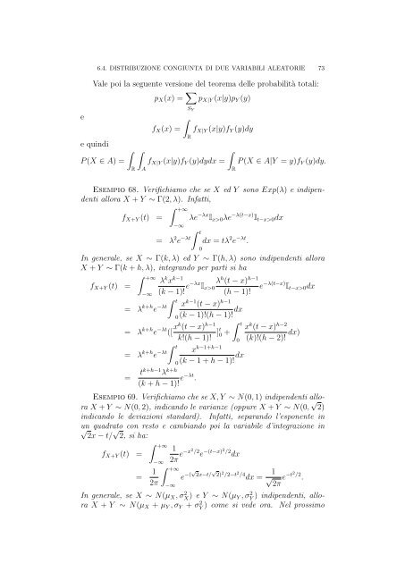
6.4. DISTRIBUZIONE CONGIUNTA DI DUE VARIABILI ALEATORIE 73Vale poi la seguente versione del teorema delle probabilità totali:p X (x) = ∑ p X|Y (x|y)p Y (y)S Yee quindi∫P (X ∈ A) =R∫A∫f X (x) =Rf X|Y (x|y)f Y (y)dy∫f X|Y (x|y)f Y (y)dydx =RP (X ∈ A|Y = y)f Y (y)dy.Esempio 68. Verifichiamo che se X ed Y sono Exp(λ) e indipendentiallora X + Y ∼ Γ(2, λ). Infatti,f X+Y (t) =∫ +∞−∞λe −λx I x>0 λe −λ(t−x) I t−x>0 dx= λ 2 e −λt ∫ t0dx = tλ 2 e −λt .In generale, se X ∼ Γ(k, λ) ed Y ∼ Γ(h, λ) sono indipendenti alloraX + Y ∼ Γ(k + h, λ), integrando per parti si haf X+Y (t) =∫ +∞−∞λ k x k−1 λ h (t − x) h−1(k − 1)! e−λx I x>0 e −λ(t−x) I t−x>0 dx(h − 1)!∫ t= λ k+h e −λt x k−1 (t − x) h−10 (k − 1)!(h − 1)! dx= λ k+h e −λt ([ xk (t − x) h−1 ∫ t] t 0 +k!(h − 1)!x k−1+h−1∫ t= λ k+h e −λt 0 (k − 1 + h − 1)! dx= tk+h−1 λ k+h(k + h − 1)! e−λt .0x k (t − x) h−2(k)!(h − 2)! dx)Esempio 69. Verifichiamo che se X, Y ∼ N(0, 1) indipendenti alloraX + Y ∼ N(0, 2), indicando le varianze (oppure X + Y ∼ N(0, √ 2)indicando le deviazioni standard). Infatti, separando l’esponente inun √ quadrato √ con resto e cambiando poi la variabile d’integrazione in2x − t/ 2, si ha:f X+Y (t) =∫ +∞= 12π−∞∫ +∞1 /22π e−x2 e −(t−x)2 /2 dx−∞e −(√ 2x−t/ √ 2) 2 /2−t 2 /4 dx = 1 √2πe −t2 /2 .In generale, se X ∼ N(µ X , σX 2 ) e Y ∼ N(µ Y , σY 2 ) indipendenti, alloraX + Y ∼ N(µ X + µ Y , σ Y + σY 2 ) come si vede ora. Nel prossimo