- Page 1 and 2:
Rock Mechanics
- Page 3 and 4:
Rock Mechanics for underground mini
- Page 5 and 6:
Contents Preface to the third editi
- Page 7 and 8:
CONTENTS 9 Excavation design in blo
- Page 9 and 10:
CONTENTS ix Appendix A Basic constr
- Page 11 and 12:
PREFACE TO THE THIRD EDITION Mining
- Page 13 and 14:
PREFACE TO THE SECOND EDITION In th
- Page 15 and 16:
PREFACE TO THE FIRST EDITION design
- Page 17 and 18:
ACKNOWLEDGEMENTS Safety in Mines Re
- Page 19 and 20:
Figure 1.1 (a) Pre-mining condition
- Page 21 and 22:
ROCK MECHANICS AND MINING ENGINEERI
- Page 23 and 24:
ROCK MECHANICS AND MINING ENGINEERI
- Page 25 and 26:
Figure 1.4 Principal features of a
- Page 27 and 28:
10 Figure 1.5 Definition of activit
- Page 29 and 30:
ROCK MECHANICS AND MINING ENGINEERI
- Page 31 and 32:
Figure 1.7 Components and logic of
- Page 33 and 34:
ROCK MECHANICS AND MINING ENGINEERI
- Page 35 and 36:
Figure 2.1 (a) A finite body subjec
- Page 37 and 38:
Figure 2.2 Free-body diagram for es
- Page 39 and 40:
STRESS AND INFINITESIMAL STRAIN As
- Page 41 and 42:
STRESS AND INFINITESIMAL STRAIN In
- Page 43 and 44:
Figure 2.3 Free-body diagram for de
- Page 45 and 46:
Figure 2.5 Problem geometry for det
- Page 47 and 48:
Figure 2.7 Rigid-body rotation of a
- Page 49 and 50:
STRESS AND INFINITESIMAL STRAIN the
- Page 51 and 52:
STRESS AND INFINITESIMAL STRAIN str
- Page 53 and 54:
⎡ ⎢ ⎣ xx yy zz xy yz zx STRES
- Page 55 and 56:
Figure 2.11 Cylindrical polar coord
- Page 57 and 58:
STRESS AND INFINITESIMAL STRAIN fre
- Page 59 and 60:
Figure 2.13 Construction of a Mohr
- Page 61 and 62:
STRESS AND INFINITESIMAL STRAIN fun
- Page 63 and 64:
3 Rock Figure 3.1 Sidewall failure
- Page 65 and 66:
Figure 3.2 Jointing in a folded str
- Page 67 and 68:
Figure 3.5 Diagrammatic longitudina
- Page 69 and 70:
Figure 3.7 Discontinuity spacing hi
- Page 71 and 72:
Figure 3.9 Illustration of persiste
- Page 73 and 74:
Figure 3.11 Typical roughness profi
- Page 75 and 76:
ROCK MASS STRUCTURE AND CHARACTERIS
- Page 77 and 78:
ROCK MASS STRUCTURE AND CHARACTERIS
- Page 79 and 80:
ROCK MASS STRUCTURE AND CHARACTERIS
- Page 81 and 82:
Figure 3.17 Sample number vs. preci
- Page 83 and 84:
Figure 3.19 Diagrammatic illustrati
- Page 85 and 86:
ROCK MASS STRUCTURE AND CHARACTERIS
- Page 87 and 88:
Figure 3.20 Computerised depiction
- Page 89 and 90:
Figure 3.23 Stereographic projectio
- Page 91 and 92:
Figure 3.26 Polar stereographic net
- Page 93 and 94:
Figure 3.28 Contours of pole concen
- Page 95 and 96:
ROCK MASS STRUCTURE AND CHARACTERIS
- Page 97 and 98:
ROCK MASS STRUCTURE AND CHARACTERIS
- Page 99 and 100:
Figure 3.30 Geological Strength Ind
- Page 101 and 102:
ROCK MASS STRUCTURE AND CHARACTERIS
- Page 103 and 104:
Figure 4.1 Idealised illustration o
- Page 105 and 106:
ROCK STRENGTH AND DEFORMABILITY wit
- Page 107 and 108:
Figure 4.4 Influence of end restrai
- Page 109 and 110:
ROCK STRENGTH AND DEFORMABILITY whe
- Page 111 and 112:
Figure 4.8 Principle of closed-loop
- Page 113 and 114:
Figure 4.12 Two classes of stress-
- Page 115 and 116:
Figure 4.14 Point load test apparat
- Page 117 and 118:
Figure 4.15 Biaxial compression tes
- Page 119 and 120:
Figure 4.18 Results of triaxial com
- Page 121 and 122:
ROCK STRENGTH AND DEFORMABILITY was
- Page 123 and 124:
Figure 4.23 Coulomb strength envelo
- Page 125 and 126:
Figure 4.25 Extension of a preexist
- Page 127 and 128:
Figure 4.29 The three basic modes o
- Page 129 and 130:
Figure 4.30 Normalised peak strengt
- Page 131 and 132:
ROCK STRENGTH AND DEFORMABILITY Tab
- Page 133 and 134:
Figure 4.32 The normality condition
- Page 135 and 136:
Figure 4.33 Variation of peak princ
- Page 137 and 138:
Figure 4.35 Direct shear test confi
- Page 139 and 140:
Figure 4.37 Shear stress-shear disp
- Page 141 and 142:
Figure 4.40 Peak and residual effec
- Page 143 and 144:
Figure 4.43 Effect of shearing dire
- Page 145 and 146: Figure 4.45 Relations between norma
- Page 147 and 148: Figure 4.47 Coulomb friction, linea
- Page 149 and 150: ROCK STRENGTH AND DEFORMABILITY whe
- Page 151 and 152: Figure 4.49 Composite peak strength
- Page 153 and 154: Figure 4.50 Hoek-Brown peak strengt
- Page 155 and 156: Figure 4.52 Determination of the Yo
- Page 157 and 158: ROCK STRENGTH AND DEFORMABILITY 4 A
- Page 159 and 160: 5 Pre-mining Figure 5.1 Method of s
- Page 161 and 162: Figure 5.2 The effect of irregular
- Page 163 and 164: PRE-MINING STATE OF STRESS surround
- Page 165 and 166: PRE-MINING STATE OF STRESS induced
- Page 167 and 168: Figure 5.5 (a) Definition of hole l
- Page 169 and 170: Figure 5.6 (a) Core drilling a slot
- Page 171 and 172: Figure 5.7 Principles of stress mea
- Page 173 and 174: PRE-MINING STATE OF STRESS strength
- Page 175 and 176: PRE-MINING STATE OF STRESS A second
- Page 177 and 178: PRE-MINING STATE OF STRESS by the e
- Page 179 and 180: PRE-MINING STATE OF STRESS extend i
- Page 181 and 182: PRE-MINING STATE OF STRESS (d) Dete
- Page 183 and 184: METHODS OF STRESS ANALYSIS quantita
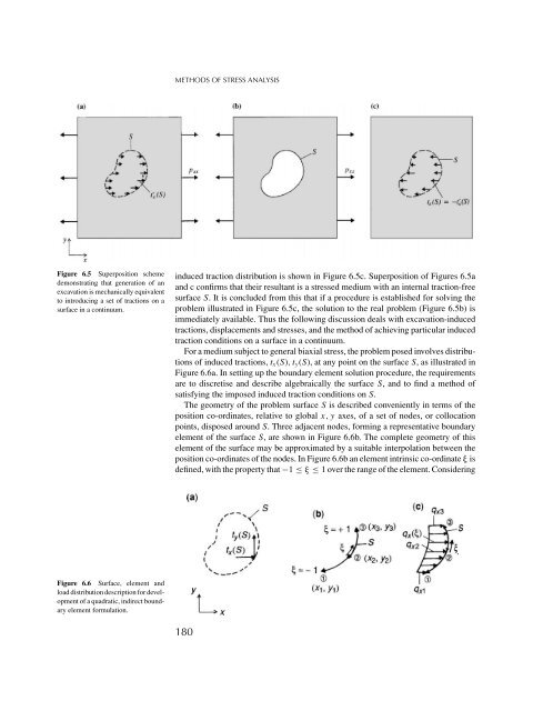
- Page 185 and 186: METHODS OF STRESS ANALYSIS It is in
- Page 187 and 188: Figure 6.2 A thick-walled cylinder
- Page 189 and 190: METHODS OF STRESS ANALYSIS For the
- Page 191 and 192: Figure 6.3 Problem geometry, coordi
- Page 193 and 194: Figure 6.4 Problem geometry, coordi
- Page 195: METHODS OF STRESS ANALYSIS When the
- Page 199 and 200: METHODS OF STRESS ANALYSIS The disc
- Page 201 and 202: Figure 6.7 Development of a finite
- Page 203 and 204: METHODS OF STRESS ANALYSIS Solution
- Page 205 and 206: Figure 6.8 A simple finite element
- Page 207 and 208: Figure 6.9 A schematic representati
- Page 209 and 210: METHODS OF STRESS ANALYSIS block ce
- Page 211 and 212: METHODS OF STRESS ANALYSIS where ˚
- Page 213 and 214: METHODS OF STRESS ANALYSIS The prin
- Page 215 and 216: EXCAVATION DESIGN IN MASSIVE ELASTI
- Page 217 and 218: Figure 7.2 A logical framework for
- Page 219 and 220: Figure 7.3 (a) Axisymmetric stress
- Page 221 and 222: Figure 7.6 A plane of weakness, ori
- Page 223 and 224: Figure 7.8 A flat-lying plane of we
- Page 225 and 226: Figure 7.10 Shear stress/normal str
- Page 227 and 228: Figure 7.12 Ovaloidal opening in a
- Page 229 and 230: Figure 7.15 States of stress at sel
- Page 231 and 232: Figure 7.16 Prediction of the exten
- Page 233 and 234: Figure 7.18 Contour plots of princi
- Page 235 and 236: Figure 7.19 Problem geometry for de
- Page 237 and 238: EXCAVATION DESIGN IN MASSIVE ELASTI
- Page 239 and 240: EXCAVATION DESIGN IN MASSIVE ELASTI
- Page 241 and 242: 8 Excavation Figure 8.1 An excavati
- Page 243 and 244: EXCAVATION DESIGN IN STRATIFIED ROC
- Page 245 and 246: Figure 8.4 Experimental apparatus f
- Page 247 and 248:
Figure 8.7 Free body diagrams and n
- Page 249 and 250:
Figure 8.8 Assumed distributions of
- Page 251 and 252:
Figure 8.9 Flow chart for the deter
- Page 253 and 254:
Figure 8.10 Normalised arch thickne
- Page 255 and 256:
EXCAVATION DESIGN IN STRATIFIED ROC
- Page 257 and 258:
Figure 8.11 Normalised deflection a
- Page 259 and 260:
9 Excavation Figure 9.1 Generation
- Page 261 and 262:
Figure 9.3 (a) A finite, non-tapere
- Page 263 and 264:
(a) (b) Figure 9.4 (a) Vertical cro
- Page 265 and 266:
(a) (b) (c) EP EP Reference circle
- Page 267 and 268:
Figure 9.10 JP 100 is the only JP w
- Page 269 and 270:
Figure 9.12 Traces of the views of
- Page 271 and 272:
EXCAVATION DESIGN IN BLOCKY ROCK In
- Page 273 and 274:
Figure 9.14 Free-body diagrams of a
- Page 275 and 276:
EXCAVATION DESIGN IN BLOCKY ROCK di
- Page 277 and 278:
Figure 9.16 Symmetrical wedge in th
- Page 279 and 280:
Figure 9.17 (a) Geometry for determ
- Page 281 and 282:
Figure 9.18 Problem geometry demons
- Page 283 and 284:
Figure 9.20 Cut-and-fill stope mine
- Page 285 and 286:
Figure 9.22 Chart to determine fact
- Page 287 and 288:
EXCAVATION DESIGN IN BLOCKY ROCK Th
- Page 289 and 290:
Figure 10.1 (a) Pre-mining state of
- Page 291 and 292:
Figure 10.3 (a) Dynamic loading of
- Page 293 and 294:
Figure 10.5 (a) Pre-mining and (b)
- Page 295 and 296:
Figure 10.6 Problem definition and
- Page 297 and 298:
ENERGY, MINE STABILITY, MINE SEISMI
- Page 299 and 300:
Figure 10.9 Force and stress compon
- Page 301 and 302:
ENERGY, MINE STABILITY, MINE SEISMI
- Page 303 and 304:
ENERGY, MINE STABILITY, MINE SEISMI
- Page 305 and 306:
ENERGY, MINE STABILITY, MINE SEISMI
- Page 307 and 308:
Figure 10.12 Distribution of radial
- Page 309 and 310:
Figure 10.15 Problem geometry for d
- Page 311 and 312:
Figure 10.17 (a) Schematic represen
- Page 313 and 314:
ENERGY, MINE STABILITY, MINE SEISMI
- Page 315 and 316:
Figure 10.20 Elastic/post-peak stif
- Page 317 and 318:
ENERGY, MINE STABILITY, MINE SEISMI
- Page 319 and 320:
Figure 10.24 Relation between frequ
- Page 321 and 322:
ENERGY, MINE STABILITY, MINE SEISMI
- Page 323 and 324:
ENERGY, MINE STABILITY, MINE SEISMI
- Page 325 and 326:
Figure 10.28 Six possible ways that
- Page 327 and 328:
Figure 10.29 First motions for P an
- Page 329 and 330:
11Rock support and reinforcement 11
- Page 331 and 332:
Figure 11.1 (a) Hypothetical exampl
- Page 333 and 334:
Figure 11.4 Non-linear support reac
- Page 335 and 336:
Figure 11.5 Idealised elastic-britt
- Page 337 and 338:
Figure 11.6 Calculated required sup
- Page 339 and 340:
ROCK SUPPORT AND REINFORCEMENT The
- Page 341 and 342:
Figure 11.9 Ground reaction curves
- Page 343 and 344:
Figure 11.12 Use of grouted reinfor
- Page 345 and 346:
ROCK SUPPORT AND REINFORCEMENT If,
- Page 347 and 348:
Figure 11.16 Local reinforcement ac
- Page 349 and 350:
Figure 11.18 Typical working sketch
- Page 351 and 352:
Figure 11.19 Permanent support and
- Page 353 and 354:
Figure 11.22 Basis of natural coord
- Page 355 and 356:
Figure 11.24 Distributions of (a) s
- Page 357 and 358:
Figure 11.26 Resin grouted rockbolt
- Page 359 and 360:
Figure 11.28 Alternative methods of
- Page 361 and 362:
ROCK SUPPORT AND REINFORCEMENT Tabl
- Page 363 and 364:
Figure 11.31 Toussaint-Heintzmann y
- Page 365 and 366:
MINING METHODS AND METHOD SELECTION
- Page 367 and 368:
Figure 12.2 Elements of a supported
- Page 369 and 370:
MINING METHODS AND METHOD SELECTION
- Page 371 and 372:
MINING METHODS AND METHOD SELECTION
- Page 373 and 374:
MINING METHODS AND METHOD SELECTION
- Page 375 and 376:
Figure 12.6 Schematic layout for bi
- Page 377 and 378:
Figure 12.8 Layout for shrink stopi
- Page 379 and 380:
Figure 12.9 Schematic layout for VC
- Page 381 and 382:
Figure 12.11 Key elements of longwa
- Page 383 and 384:
Figure 12.13 Mining layout for tran
- Page 385 and 386:
MINING METHODS AND METHOD SELECTION
- Page 387 and 388:
13 Figure 13.1 Schematic illustrati
- Page 389 and 390:
Figure 13.3 Layout of barrier pilla
- Page 391 and 392:
Figure 13.5 Principal modes of defo
- Page 393 and 394:
Figure 13.8 Geometry for tributary
- Page 395 and 396:
PILLAR SUPPORTED MINING METHODS str
- Page 397 and 398:
Figure 13.10 Distribution of vertic
- Page 399 and 400:
Figure 13.12 Pillar behaviour domai
- Page 401 and 402:
PILLAR SUPPORTED MINING METHODS Lun
- Page 403 and 404:
Figure 13.15 Options in the design
- Page 405 and 406:
Figure 13.17 Relation between yield
- Page 407 and 408:
Figure 13.19 Model of yield of coun
- Page 409 and 410:
Figure 13.20 North-south vertical c
- Page 411 and 412:
Figure 13.23 Stope-and-pillar layou
- Page 413 and 414:
Figure 13.25 Calibrated stability c
- Page 415 and 416:
PILLAR SUPPORTED MINING METHODS wor
- Page 417 and 418:
Figure 13.28 Pillar performance, de
- Page 419 and 420:
Figure 13.29 (a) Stope and pillar l
- Page 421 and 422:
Figure 13.31 (a) Plane strain analy
- Page 423 and 424:
PILLAR SUPPORTED MINING METHODS Pan
- Page 425 and 426:
14 Artificially supported mining me
- Page 427 and 428:
ARTIFICIALLY SUPPORTED MINING METHO
- Page 429 and 430:
ARTIFICIALLY SUPPORTED MINING METHO
- Page 431 and 432:
Figure 14.2 Simplified view of stru
- Page 433 and 434:
ARTIFICIALLY SUPPORTED MINING METHO
- Page 435 and 436:
Figure 14.5 Confined block model fo
- Page 437 and 438:
Figure 14.7 Crown and sidewall stre
- Page 439 and 440:
ARTIFICIALLY SUPPORTED MINING METHO
- Page 441 and 442:
ARTIFICIALLY SUPPORTED MINING METHO
- Page 443 and 444:
Figure 14.10 Sublevel open stoping
- Page 445 and 446:
Figure 14.12 Some applications of c
- Page 447 and 448:
15 Longwall and caving mining metho
- Page 449 and 450:
Figure 15.2 Shear stress drop in th
- Page 451 and 452:
LONGWALL AND CAVING MINING METHODS
- Page 453 and 454:
LONGWALL AND CAVING MINING METHODS
- Page 455 and 456:
Figure 15.6 Hydraulic prop reaction
- Page 457 and 458:
Figure 15.7 Development and extract
- Page 459 and 460:
Figure 15.8 Vertical stress redistr
- Page 461 and 462:
Figure 15.11 Distribution of observ
- Page 463 and 464:
Figure 15.13 Plan view of microseis
- Page 465 and 466:
Figure 15.16 Ground-support interac
- Page 467 and 468:
Figure 15.18 Roadway support and re
- Page 469 and 470:
LONGWALL AND CAVING MINING METHODS
- Page 471 and 472:
LONGWALL AND CAVING MINING METHODS
- Page 473 and 474:
LONGWALL AND CAVING MINING METHODS
- Page 475 and 476:
Figure 15.25 Comparison of isolated
- Page 477 and 478:
Figure 15.26 Geometry of a sublevel
- Page 479 and 480:
Figure 15.28 Theoretical determinat
- Page 481 and 482:
Figure 15.31 Deterioration of a cro
- Page 483 and 484:
Figure 15.32 Distinct element simul
- Page 485 and 486:
LONGWALL AND CAVING MINING METHODS
- Page 487 and 488:
Figure 15.34 Extended Mathews stabi
- Page 489 and 490:
Figure 15.36 Comparison of postand
- Page 491 and 492:
LONGWALL AND CAVING MINING METHODS
- Page 493 and 494:
Figure 15.39 Idealised plan illustr
- Page 495 and 496:
Figure 15.41 Idealised vertical sec
- Page 497 and 498:
Figure 15.42 Vertical slice through
- Page 499 and 500:
LONGWALL AND CAVING MINING METHODS
- Page 501 and 502:
16 Figure 16.1 Trough subsidence ov
- Page 503 and 504:
MINING-INDUCED SURFACE SUBSIDENCE c
- Page 505 and 506:
Figure 16.4 North-south section, At
- Page 507 and 508:
Figure 16.6 (a) Rectangular block g
- Page 509 and 510:
MINING-INDUCED SURFACE SUBSIDENCE f
- Page 511 and 512:
Figure 16.8 Relation between stope
- Page 513 and 514:
MINING-INDUCED SURFACE SUBSIDENCE M
- Page 515 and 516:
MINING-INDUCED SURFACE SUBSIDENCE
- Page 517 and 518:
Figure 16.14 Chart developed to est
- Page 519 and 520:
Figure 16.16 Progressive hangingwal
- Page 521 and 522:
Figure 16.19 Idealised model used i
- Page 523 and 524:
Figure 16.21 Longitudinal section,
- Page 525 and 526:
MINING-INDUCED SURFACE SUBSIDENCE t
- Page 527 and 528:
MINING-INDUCED SURFACE SUBSIDENCE w
- Page 529 and 530:
MINING-INDUCED SURFACE SUBSIDENCE F
- Page 531 and 532:
Figure 16.25 Subsidence troughs pre
- Page 533 and 534:
Figure 16.28 Predicted and measured
- Page 535 and 536:
17 Blasting mechanics 17.1 Blasting
- Page 537 and 538:
Figure 17.1 An empirical matching o
- Page 539 and 540:
Figure 17.2 A finite difference mod
- Page 541 and 542:
Figure 17.4 Reflection of a cylindr
- Page 543 and 544:
BLASTING MECHANICS means that no ci
- Page 545 and 546:
Figure 17.8 Layout of blast holes i
- Page 547 and 548:
Figure 17.9 Influence of field stat
- Page 549 and 550:
Figure 17.11 Generation of surface
- Page 551 and 552:
BLASTING MECHANICS The components o
- Page 553 and 554:
BLASTING MECHANICS amplitudes of th
- Page 555 and 556:
BLASTING MECHANICS 17.9 Evaluation
- Page 557 and 558:
Figure 17.15 (a) Schematic cross se
- Page 559 and 560:
BLASTING MECHANICS in Figure 17.17,
- Page 561 and 562:
MONITORING ROCK MASS PERFORMANCE (a
- Page 563 and 564:
MONITORING ROCK MASS PERFORMANCE su
- Page 565 and 566:
MONITORING ROCK MASS PERFORMANCE Ta
- Page 567 and 568:
Figure 18.2 The Distometer ISETH, a
- Page 569 and 570:
Figure 18.5 Self-inductance multipl
- Page 571 and 572:
MONITORING ROCK MASS PERFORMANCE is
- Page 573 and 574:
Figure 18.9 Biaxial vibrating wire
- Page 575 and 576:
MONITORING ROCK MASS PERFORMANCE me
- Page 577 and 578:
Figure 18.12 Cross section at 6650N
- Page 579 and 580:
Figure 18.13 Examples of convergenc
- Page 581 and 582:
Figure 18.15 Longitudinal section l
- Page 583 and 584:
Figure 18.16 (Cont.) MONITORING ROC
- Page 585 and 586:
Appendix A Basic constructions usin
- Page 587 and 588:
Figure A.3 Determining the angle be
- Page 589 and 590:
APPENDIX A USE OF HEMISPHERICAL PRO
- Page 591 and 592:
APPENDIX B STRESSES AND DISPLACEMEN
- Page 593 and 594:
Figure A.6 Axisymmetric tunnel prob
- Page 595 and 596:
Figure A.9 Bolt load-extension curv
- Page 597 and 598:
APPENDIX D LIMITING EQUILIBRIUM ANA
- Page 599 and 600:
APPENDIX D LIMITING EQUILIBRIUM ANA
- Page 601 and 602:
APPENDIX D LIMITING EQUILIBRIUM ANA
- Page 603 and 604:
ANSWERS TO PROBLEMS 2 (a) 0.087 - 0
- Page 605 and 606:
ANSWERS TO PROBLEMS 3 wp = 38.6 m,
- Page 607 and 608:
REFERENCES Symp. & 17th Tunn. Assn
- Page 609 and 610:
REFERENCES Brady, B. H. G. and Bray
- Page 611 and 612:
REFERENCES Collier, P. A. (1993) De
- Page 613 and 614:
REFERENCES Drescher, A. and Vardoul
- Page 615 and 616:
REFERENCES Gustafsson, P. (1998) Wa
- Page 617 and 618:
REFERENCES Hood, M. and Brown, E. T
- Page 619 and 620:
REFERENCES Kaiser, P. K. and Tannan
- Page 621 and 622:
REFERENCES Lorig, L. J. and Brady,
- Page 623 and 624:
REFERENCES Ortlepp, W. D. (1994) Gr
- Page 625 and 626:
REFERENCES Rojas, E., Molina, R. an
- Page 627 and 628:
REFERENCES Spottiswoode, S. M. and
- Page 629 and 630:
REFERENCES Villaescusa, E., Windsor
- Page 631 and 632:
Index Page numbers appearing in bol
- Page 633 and 634:
INDEX Coulomb (cont.) parameters 96
- Page 635 and 636:
INDEX Excavation (cont.) support ra
- Page 637 and 638:
INDEX Jaeger’s plane of weakness
- Page 639 and 640:
INDEX Panel caving 470-2, 473, 474,
- Page 641 and 642:
INDEX Seismic (cont.) moment 306, 3
- Page 643 and 644:
INDEX Strength (cont.) residual 86,
- Page 645:
INDEX United States (USA) 395, 396,