Rotational Raman scattering in the Earth's atmosphere ... - SRON

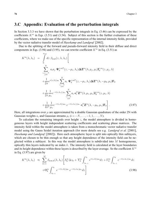
76 Chapter 3
3.C Appendix: Evaluation of the perturbation integrals
In Section 3.3.3 we have shown that the perturbation integrals in Eq. (3.46) can be expressed by the
coefficients K m in Eqs. (3.51) and (3.54). Subject of this section is the further evaluation of these
coefficients, where we make use of the specific representation of the internal intensity fields, provided
by the vector radiative transfer model of Hasekamp and Landgraf [2002].
Due to the splitting of the forward and pseudo-forward intensity field in their diffuse and direct
components in Eqs. (3.94) and (3.95), we can rewrite coefficient K m in Eq. (3.51) as
∫z top
[
K m (λ,λ v ) = dz β scat (z,λ,λ v )
0
N∑
i,j=−N
j≠0
a i a j Ψ +mT
d
(z, −µ i ,λ v )∆Z m (λ,µ j ,µ i )I +m
d
(z,µ j ,λ)
+ 1
2π eτ(z,λ)/µ 0
+ 1
2π
N∑
i=−N
i≠0
1 ∑ N
e −τ(z,λv)/µv
µ v
a i Ψ +mT
d
(z, −µ i ,λ v )∆Z m (λ, −µ 0 ,µ i )F 0
i=−N
i≠0
a i e T i Z m (λ,µ i ,µ v )I +m
d
(z,µ i ,λ)
]
+ 1 1
e −τ(z,λ)/µ 0
e −τ(z,λv)/µv e T
4π 2 i Z m (λ, −µ 0 ,µ v )F 0
µ v
. (3.97)
Here, all integrations over µ are approximated by a double Gaussian quadrature of the order 2N with
Gaussian weights a i and Gaussian streams µ i (i=−N,...,−1, 1,...,N).
To calculate the remaining integrals over height z, the model atmosphere is divided in homogeneous
layers with height independent scattering coefficients and scattering phase matrices. The
intensity field within the model atmosphere is taken from a monochromatic vector radiative transfer
model using the Gauss Seidel iteration approach (for more details see e.g. Landgraf et al. [2001],
Hasekamp and Landgraf [2002]). Here each atmospheric layer is split into optically thin sublayers,
which are chosen to be thin enough so that any height dependence of the intensity field can be neglected
within a sublayer. In this way the model atmosphere is subdivided into M homogeneous,
optically thin layers indicated by an index k. The intensity field is calculated at the layer boundaries
and its height dependence within these layers is described by the layer average. So the coefficient K m
in Eq. (3.97) are given by
[
M∑
∫ zk
∫ zk
K m (λ,λ v ) ≈ β scat,k (λ,λ v ) Λ m k ∆z k + Υ m k e τ(z,λ)/µ 0
dz + Γ m k e −τ(z,λv)/µv dz
k=1
z k−1 z k−1
]
+Θ m k
∫ zk
z k−1
e −τ(z,λ)/µ 0
e −τ(z,λv)µv dz
(3.98)