FIBEROPTIC SENSOR TECHNOLOGY HANDBOOK
FIBEROPTIC SENSOR TECHNOLOGY HANDBOOK
FIBEROPTIC SENSOR TECHNOLOGY HANDBOOK

You also want an ePaper? Increase the reach of your titles
YUMPU automatically turns print PDFs into web optimized ePapers that Google loves.
sors or a pressure gradient sensor. Sensor arrays will<br />
be considered in Chapter 6. Pressure gradient hydrophores<br />
sense the pressure at two closely spaced points.<br />
The distance between sensors, S, iS typically much less<br />
than the wavelength of sound, k, in the propagation<br />
medium, namely water in the calculations that follow.<br />
A pressure gradient measurement can be accomplished by<br />
means of either two distinct sensors, one at each point,<br />
or by a single senaor apanning the distance between the<br />
two points. Both types of sensora will be considered<br />
here.<br />
Since the output signal from a pressure-gradient<br />
hydrophore is proportional to the preasure gradient,<br />
ita reaponse ia proportional to the particle velocity.<br />
Such sensors are therefore often called particle<br />
velocity hydrophores. This is an advantage when operating<br />
near a pressure releaae aurface where the particle<br />
velocity almost doublea and the pressure itself goes to<br />
zero. The tendency to reapond to particle velocity<br />
renders them more aensitive to flow noiae than omnidirectional<br />
hydrophores. Thia follows because particle<br />
velocity fluctuations associated with flow are often<br />
much greater than the particle velocity oscillations<br />
associated with the acoustic signal being measured.<br />
Consider the sine wave shown in Fig. 5.8 where the<br />
Fig. 5.9<br />
100<br />
90<br />
80<br />
70<br />
60<br />
50<br />
40<br />
30<br />
20<br />
\<br />
1<br />
3 5 ID 2 5 100 2 5 1,000 2 5 10,000<br />
FREOUENCY (Hz)<br />
HEAVY<br />
SS2 WIND<br />
SPEED<br />
10 KTS<br />
RAIN<br />
V a r i a t i o n of the acouatic energy spectrum<br />
level aa a function of frequency for a fiberoptic<br />
presaure-gradient hydrophore with<br />
other noise levels in a sea subsurface environment.<br />
P<br />
PA- -<br />
I<br />
The calculated reaults shown in Fig. 5.9 is<br />
for the case of the aound wave propagating parallel to<br />
the line joining the two sensors. The sensitivity of<br />
a Preasure gradient sensor to a sound wave propagating<br />
perpendicular to this direction ia zero because both<br />
sensors are then aubjected to the aame pressure. The<br />
directivity is dipole-like aa shown in Fig. 5.10(a).<br />
The cardioid directional responae shown in Fig. 5.10(b)<br />
can be obtained by combining the dipole output with<br />
that of an omnidirectional hydrophore with sensitivity<br />
equal to that exhibited by the dipole at e = OO. The<br />
Fig. 5.8<br />
The pressure distribution aa a function of<br />
distance from the zero-preasure point of a<br />
single pressure wave.<br />
instantaneous acoustic preasure, P, is given by:<br />
p = pAsiI’i (2~/ka)x (5.10)<br />
where pA is the acoustic amplitude, as is the sound<br />
wavelength, and x is distance in the same units as ~.<br />
The pressure amplitude at x = O and x = S (S