Local polarization dynamics in ferroelectric materials

Rep. Prog. Phys. 73 (2010) 056502
S V Kalinin et al
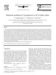
Figure 7. Relation between ideal image and experimental image in real and Fourier spaces. Object transfer function is a Fourier transform
of resolution function. Reproduced from [197]. Copyright 2006, IOP Publishing.
where I(q) = ∫ I(x)e iqx dx, I 0 (q) and N(q) are the Fourier
transforms of the measured image, ideal image and noise,
respectively. The object transfer function (OTF), F(q), is
defined as a Fourier transform of the resolution function, F(y).
The object transfer function, F(q), and the resolution function,
F(y), can then be determined directly provided that the ideal
image, I 0 (q), is known. Alternatively, the resolution function
can be approximated assuming that some information on its
functional behavior (e.g. function is monotonic) is available
(blind reconstruction, Bayesian methods). The veracity of this
determination is limited by the noise level, N(q). Then, once
the resolution function is determined for a known calibration
standard, it can be used to extract the ideal image, I 0 (x),
from a measured image, I(x), for an arbitrary sample. The
relationship between the ideal image, experimental image and
resolution and object transfer functions is illustrated in figure 7.
For the PFM OTF shown in figure 6(c), two parameters
describing resolution can be introduced. The first definition
can be derived from the Rayleigh or 25–75 criteria [198].
This Rayleigh two-point resolution (RTR) establishes a
conservative definition of resolution as a characteristic object
size for which response can still be measured quantitatively. In
comparison, the information limit defines the minimum feature
size that can still be detected qualitatively in the presence of
noise, as illustrated in figure 6(d).
Beyond definition of resolution, equations (2.9a) and
(2.9b) suggest an approach to deconvolute the ideal image
assuming that the resolution function is known or can be
estimated. Note that direct deconvolution results in a spurious
increase in the noise amplitude, necessitating the use of
regularization methods that impose the constraints on the
maximum roughness of the ideal image. Detailed analysis
of the inverse imaging problem is available in the literature
[199] and a number of commercial packages are available
(MatLab, DigitalMicrograph). Furthermore, a number of
references analyzing deconvolution theory in Kelvin probe
force microscopy (KPFM), a technique closely related to PFM,
have been reported [200].
2.3.2. Phenomenological resolution theory in PFM
2.3.2.1. Determining resolution. The OTF and information
limit in PFM can be determined (a) using the analysis of the
Fourier transforms (diffractograms) of periodic structures and
(b) domain wall profiles. Periodic domain structures can be
either created by writing or occur naturally, as in lamellar
(a)–(c) domains of tetragonal ferroelectrics. Figure 8(a) shows
the template pattern used to write domains on the PZT surface
along with the corresponding diffractogram. For comparison,
shown in figures 8(c) and (d) are the resultant domain patterns
imaged by PFM and their Fourier transforms. Note that only a
few low order reflections can be observed in the diffractogram
as a consequence of finite instrumental resolution.
To illustrate the effect of imaging conditions on the
PFM resolution, it is instructive to explore the effect of
lock-in time constant, as studied in detail in [197] and is
illustrated in figures 8(b)–(e). Imaging with a low time
constant (0.5 ms) results in a sharp, but relatively noisy,
image (as seen in both the real space and FT images). On
increasing the time constant to 1 ms, the noise level decreases.
However, increasing the time constant further, to 4, 10 and
20 ms, results in characteristic streaking in real-space images
along the fast scan direction. Note the evolution of the
noise background in the corresponding diffractograms from
a rotationally isotropic noise pattern for small time constants
(figures 8(b) and (c)) to a pronounced noise band for large
time constants in figures 8(d)–(e), indicating a large anisotropy
of noise in the slow and fast scan directions. Also note that
despite the high smearing in figure 8(e) from the large time
constant (the pattern is not visually discernible in the realspace
image), the corresponding diffractogram still contains
reflections corresponding to the written pattern.
The wave-vector dependence of the peak intensity of
several (hk) reflections for different lock-in time constants
is shown in figure 8(f ). The peak intensities follow an
exponential decay law, I (hk) = I 0 exp(−q/G), where the
decay constant is independent of the lock-in settings, G ≈
5 µm −1 , q = √ h 2 + k 2 /a and a is the periodicity of the lattice.
Thus, the intensity of the (1 0) peak can be used as a measure of
the overall peak-to-noise ratio of the diffractogram, and hence
of the image quality. A plot of the intensity of the (1 0) peak
as a function of lock-in settings is given in figure 8(g). The
peak intensity is virtually constant for small time constants and
rapidly becomes zero when the time constant becomes larger
than the time corresponding to the pixel acquisition rate (5 ms),
reflecting the evolution of image contrast in figure 8.
The experimental resolution function can be determined
from the diffractogram as shown in figure 9. Note that the
resolution and contrast transfer function above are defined
10