Local polarization dynamics in ferroelectric materials

Rep. Prog. Phys. 73 (2010) 056502
S V Kalinin et al
Intensity, a.u.
10 -1
10 -2
1 ms
5 ms
10 ms
(1,1) Peak Intensity
0.10
0.05
(f)
0.005 0.010
Wavevector, nm -1
(g)
0.00
1 10
Lock-in time constant, ms
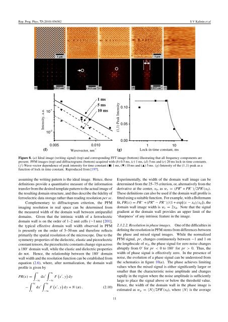
Figure 8. (a) Ideal image (writing signal) (top) and corresponding FFT image (bottom) illustrating that all frequency components are
present. PFM images (top) and diffractograms (bottom) acquired with (b) 0.5 ms, (c) 1 ms, (d) 5 ms and (e) 20 ms lock-in time constants.
(f ) Wave-vector dependence of peak intensity for time constant ( ) 1 ms, () 10 ms and () 5 ms. (g) Intensity of the (1 ,1) peak as a
function of lock-in time constant. Reproduced from [197].
assuming the writing pattern is the ideal image. Hence, these
definitions provide a quantitative measure of the information
transfer from the desired template pattern to the actual image of
the resulting domain structure, and thus describe the fidelity of
ferroelectric data storage rather than reading resolution per se.
Complementary to diffractogram criterion, the PFM
imaging resolution in real space can be determined from
the measured width of the domain wall between antiparallel
domains. Given that the intrinsic width of a ferroelectric
domain wall is on the order of 1–2 unit cells (∼1 nm) [201],
the typical effective domain wall width observed in PFM
is presently on the order of 5–50 nm and therefore reflects
primarily the spatial resolution of the microscope. Due to the
symmetry properties of the dielectric, elastic and piezoelectric
constant tensors, the piezoelectric constants change sign across
a 180 ◦ domain wall, while the elastic and dielectric properties
do not. Hence, the relationship between the 180 ◦ domain
wall width and the resolution function can be established from
equation (2.6), where, after normalization, the domain wall
profile is given by
∫ x ∫ ∞
PR(x) = dx ′ F ( x ′ ,y ) dy
−
−∞
∫ ∞
x
−∞
∫ ∞
dx ′ F ( x ′ ,y ) dy + N (x) . (2.10)
−∞
Experimentally, the width of the domain wall image can be
determined from the 25–75 criterion, or, alternatively from the
derivative at the center, x 0 ,asw r = (PR + + PR − )/2PR ′ (x 0 ).
These definitions can also be used if the domain wall profile is
fitted using a suitable function. For example, with a Boltzmann
fit, PR(x) = PR − + (PR + − PR − )/(1+exp[(x − x 0 )/x d ]), the
domain wall image width is w r = 2x d . Note that the signal
gradient at the domain wall provides an upper limit of the
‘sharpness’ of any intrinsic feature in the image.
2.3.2.2. Resolution in phase images. One of the difficulties in
defining the resolution in PFM stems from differences between
the phase and mixed signal images. While the normalized
PFM signal, pr, changes continuously between −1 and1on
the lengthscale of w d , the phase signal for zero noise changes
abruptly from 0 ◦ for pr < 0 to 180 ◦ for pr > 0. Thus, the
width of phase signal is effectively zero. In the presence of
noise, the evolution of a phase signal can be understood from
the schematics in figure 10(a). The phase achieves limiting
values when the mixed signal is either significantly larger or
smaller than the characteristic noise amplitude and changes
rapidly in the region where the noise amplitude is sufficiently
large to place the signal above or below the threshold value.
Hence, the width of the domain wall in the phase image is
estimated as w ϕ =〈N〉/2PR ′ (x 0 ), where 〈N〉 is the average
11