Local polarization dynamics in ferroelectric materials

Rep. Prog. Phys. 73 (2010) 056502
S V Kalinin et al
d33 eff (pm/V)
80
3
40
4
0
-40
1
2
-80
(a)
10 -3 10 -2 0.1 1 10 10 2
r/R 0
d33 eff (normalized)
d33 eff (pm/V)
1.
0.5
0.
-0.5
-1
10 -3 10 -2 0.1 1 10 10 2
r/R 0
80 3
40
0
(c)
-40 1
2
-80
10 -3 10 -2 0.1 1 10 10 2
r/d
(b)
4
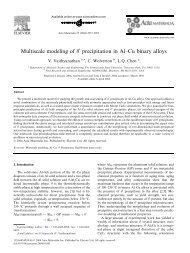
Figure 16. Absolute (a), (c) and normalized (b) piezoresponse d33 eff (r) versus the domain radius for the point charge (c) and sphere–plane
(a), (b) models of the tip at ν = 0.35 for BTO (1), PZT6B (2), PTO (3), LNO (4). Reproduced from [186]. Copyright 2007, American
Institute of Physics.
h Pade
2.3.4.4. Response of axially symmetric cylindrical domain.
The deconvolution of PFM spectroscopy data requires analysis
−2
1+2γ
(1+γ ) 2 − 2 (1+ν) s
1+γ s + π/8 , (2.24b)
of the PFM signal from a finite domain centered at the tip apex,
as shown in figure 14(b). For most ferroelectric materials,
domains form highly elongated needles extending deep into
the material, whereas the electrostatic field is concentrated in
the near-surface region. Hence, interpretation of PFM data
can be performed using a model of a semi-infinite cylindrical
domain. Hence, the response can be estimated assuming that
the domain wall is purely cylindrical and the charged tip is
located at the domain center (0,0,0). From equation (2.15),
the displacement at the center of a domain is
(∫ ∞
∫ r
)
u 3 (0,r)=2π ρdρW 3jkl (ρ)−2
0
0
ρdρW 3jkl (ρ) d lkj .
(2.22)
Here the resolution
√
function, W 3jkl (ρ), is given by
equation (2.16) for ξ1 2 + ξ 2 2 = ρ, while u 1 = u 2 = 0as
follows from the symmetry considerations. Both for the point
charge and the sphere–plane models, the vertical displacement
can be obtained in a simple analytical form as
⎧
Q
( r
)
2πε 0 (ε e + κ) d hPade jk
d ,γ,ν d kj ,
⎪⎨
point charge model,
u 3 = ( )
(2.23)
r
Uh Pade
jk
,γ,ν d kj ,
⎪⎩
fR 0
sphere–plane model.
Integral representations for functions h jk (s,γ,ν)are derived
in [186]. Their polynomial and exponential Pade
approximations are derived in [186]. For γ ∼ = 1 and s>0.1
the following simple approximations are obtained:
h Pade
33 (s, γ) ≈− 1+2γ 1+2γ
+2
2
(1+γ ) (1+γ ) 2 · s
s + π/8 , (2.24a)
h Pade
13 (s, γ, ν) ≈ 1+2γ
(1+γ ) 2 − 2 (1+ν)
1+γ
(
)
51 (s, γ) ≈− γ 2
(1+γ ) 2 +2 γ 2
(1+γ ) 2 ·
s 2
2 γ 2
(1+γ ) 2 +5πs/8+s 2 .
(2.24c)
For good tip–surface contact, the piezoresponse signal is d33 eff =
u 3 (r)/U and can be written as d33 eff = h 13d 31 + h 51 d 15 + h 33 d 33 .
Piezoresponse d33 eff (r) versus the cylindrical domain radius
for the sphere–plane and point charge models of the tip
for different ferroelectric materials is shown in figure 16.
Similarly to domain wall imaging, the best sensitivity to small
domains formed below the tip can be achieved in BTO, whereas
the worst one corresponds to LNO independently of the tip
representation.
From the data in figure 16, the coercive bias in the PFM
hysteresis loop measurements (i.e. when the response is zero,
corresponding to equality of the PFM signal from the nascent
domain and the surrounding unswitched matrix) in the point
contact approximation corresponds to a domain size of the
order of 0.1R 0 (for BTO) to 0.7R 0 (for PZT6B and LNO).
This suggests that the early steps of the switching process are
local, i.e. the information is collected from the area below the
characteristic tip size. Furthermore, the significant (∼10%)
deviations of the PFM signal from constant begin for domain
sizes well below (factor of 10–30) the characteristic tip size.
Therefore, the initial nucleation stages can be probed even
when the domain is extremely small (on the order of several
nanometers (for R 0 = 50 nm)). On the other hand, the
response saturates fairly slowly with the domain size, and
hence the ‘tails’ of the hysteresis loop contain information on
domain sizes well above the tip size.
To summarize, the analytical expressions equations (2.23)
and (2.24a)–(2.24c) relate the piezoresponse signal measured
at the center of the domain d33 eff (r) and the domain radius.
This allows the domain radius–voltage dependence r(U) to be
reconstructed from the experimental data of the piezoresponse
hysteresis d33 eff (U) once the tip parameters are determined using
an appropriate calibration procedure (e.g. from the domain wall
profile).
18