Local polarization dynamics in ferroelectric materials
Local polarization dynamics in ferroelectric materials
Local polarization dynamics in ferroelectric materials

You also want an ePaper? Increase the reach of your titles
YUMPU automatically turns print PDFs into web optimized ePapers that Google loves.
Rep. Prog. Phys. 73 (2010) 056502<br />
S V Kal<strong>in</strong><strong>in</strong> et al<br />
Figure 4. The dependence of (a) displacement u 3 ,(b) piezoelectric tensor component e 33 , for PbTiO 3 (PTO, ν = 0.3 (Poisson’s ratio)) on<br />
Euler’s angle θ <strong>in</strong> the laboratory coord<strong>in</strong>ate system. The dependence of (c) piezoelectric tensor component e 33 and (d) displacement u 3 for<br />
LiTaO 3 (LTO, ν = 0.25) on Euler’s angles ϕ, θ <strong>in</strong> the laboratory coord<strong>in</strong>ate system. Reproduced from [185]. Copyright 2007, American<br />
Institute of Physics.<br />
trigonal LiTaO 3 (LTO) model systems <strong>in</strong> figure 4. Note<br />
that while <strong>in</strong> this analysis, the dielectric properties of the<br />
material are assumed to be close to isotropic and hence the<br />
electric field distribution is <strong>in</strong>sensitive to sample orientation,<br />
similar analysis can be performed for full dielectric and elastic<br />
anisotropy.<br />
The dependence of the piezoelectric tensor component e 35<br />
versus the orientation of the crystallographic axes with respect<br />
to the laboratory coord<strong>in</strong>ate system for a LTO crystal is shown<br />
<strong>in</strong> the upper row of figure 5. The horizontal displacement<br />
below the tip versus the orientation of the crystallographic<br />
axes with respect to the laboratory coord<strong>in</strong>ate system for a<br />
LTO crystal is shown <strong>in</strong> the bottom row of figure 5.<br />
A common feature of the displacement surfaces shown <strong>in</strong><br />
figures 4 and 5 is that the u 1 angular distribution is smoother,<br />
much more symmetric and convex than the one for e 35 .<br />
Similarly to the longitud<strong>in</strong>al components of the piezoelectric<br />
tensors e 33 and d 33 , the d 35 surfaces are very similar to e 35<br />
surfaces.<br />
2.3. Resolution theory <strong>in</strong> PFM<br />
One of the basic parameters characteriz<strong>in</strong>g performance of<br />
a microscope is the spatial resolution. Despite the ubiquity<br />
of usage and ‘<strong>in</strong>tuitive’ mean<strong>in</strong>g, the resolution <strong>in</strong> SPM is<br />
typically def<strong>in</strong>ed ad hoc. A quantitative imag<strong>in</strong>g theory <strong>in</strong><br />
PFM (and other SPMs) is required <strong>in</strong> order to:<br />
• def<strong>in</strong>e the resolution and <strong>in</strong>formation limits <strong>in</strong> PFM and<br />
establish their dependence on tip geometry and <strong>materials</strong><br />
properties, hence suggest<strong>in</strong>g strategies for high-resolution<br />
imag<strong>in</strong>g;<br />
• develop the pathways for calibration of tip geometry <strong>in</strong><br />
the PFM experiment for quantitative data <strong>in</strong>terpretation;<br />
• <strong>in</strong>terpret the imag<strong>in</strong>g and spectroscopy data <strong>in</strong> terms of<br />
<strong>in</strong>tr<strong>in</strong>sic doma<strong>in</strong> wall widths and the size of the nascent<br />
doma<strong>in</strong> below the tip;<br />
• reconstruct the ideal image from experimental data<br />
(deconvolute tip contribution), and establish applicability<br />
limits and errors associated with such deconvolution<br />
processes.<br />
In this section, we describe the basic pr<strong>in</strong>ciples of l<strong>in</strong>ear<br />
imag<strong>in</strong>g theory, provide def<strong>in</strong>itions of resolution and<br />
<strong>in</strong>formation limit and describe <strong>in</strong>strumental and theoretical<br />
aspects of resolution function theory <strong>in</strong> PFM.<br />
2.3.1. L<strong>in</strong>ear imag<strong>in</strong>g theory: transfer function, resolution<br />
and <strong>in</strong>formation limit. The def<strong>in</strong>ition of spatial resolution<br />
and resolution theory have orig<strong>in</strong>ally evolved <strong>in</strong> the context of<br />
optical and electron microscopy (EM). In optics, the Rayleigh<br />
criterion [196] def<strong>in</strong>es the resolution as the m<strong>in</strong>imum distance<br />
by which two po<strong>in</strong>t scatterers must be separated <strong>in</strong> order to<br />
be discernible for a given imag<strong>in</strong>g system. A commonly<br />
used alternative read<strong>in</strong>g of the criterion postulates that for<br />
two Gaussian-shaped image features of similar <strong>in</strong>tensity to be<br />
resolved, the dip between the two maxima should be at least<br />
21% of the maximum. This criterion is illustrated <strong>in</strong> figure 6(a)<br />
and shows the transition of the two features from completely<br />
resolved to unresolved as a function of the separat<strong>in</strong>g distance.<br />
Note that the criterion is not absolute. It is possible that for<br />
a system with a sufficiently high signal-to-noise ratio, peaks<br />
separated by less than Rayleigh’s resolution can be discernible<br />
8