Local polarization dynamics in ferroelectric materials
Local polarization dynamics in ferroelectric materials
Local polarization dynamics in ferroelectric materials

You also want an ePaper? Increase the reach of your titles
YUMPU automatically turns print PDFs into web optimized ePapers that Google loves.
Rep. Prog. Phys. 73 (2010) 056502<br />
S V Kal<strong>in</strong><strong>in</strong> et al<br />
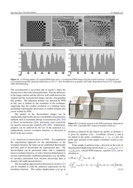
Figure 11. (a) Writ<strong>in</strong>g pattern, (b) orig<strong>in</strong>al PFM image and (c) reconstructed PFM image us<strong>in</strong>g the transfer function. (d) Orig<strong>in</strong>al and<br />
(e) reconstructed profiles along the dashed l<strong>in</strong>es <strong>in</strong> (b), (c). Note the difference <strong>in</strong> doma<strong>in</strong> wall width. Reproduced from [197]. Copyright<br />
2006, IOP Publish<strong>in</strong>g.<br />
The reconstruction is successful only <strong>in</strong> region I, where the<br />
doma<strong>in</strong> size is above the <strong>in</strong>formation limit. Note the difference<br />
<strong>in</strong> the image contrast and the effective wall width between the<br />
orig<strong>in</strong>al and the reconstructed images and the correspond<strong>in</strong>g<br />
l<strong>in</strong>e profiles. The m<strong>in</strong>imum doma<strong>in</strong> size detected by PFM<br />
<strong>in</strong> this case is limited by the resolution of the technique,<br />
suggest<strong>in</strong>g that the read<strong>in</strong>g resolution is a limit<strong>in</strong>g factor<br />
preclud<strong>in</strong>g experimental observation of smaller doma<strong>in</strong>s that<br />
can be written by PFM.<br />
The quality of the deconvoluted images can be<br />
significantly improved by the use of probability-based iterative<br />
methods such as maximum entropy reconstruction [202, 203]<br />
or Pixon reconstruction [204], previously used extensively<br />
for electron microscopic methods [205, 206]. Furthermore,<br />
progress can be achieved by the use of the analytical (i.e.<br />
<strong>in</strong>dependently known) resolution function, as discussed <strong>in</strong><br />
detail <strong>in</strong> the next section.<br />
2.3.3. Analytical resolution theory <strong>in</strong> PFM. To complement<br />
the experimental approach for the determ<strong>in</strong>ation of the<br />
resolution function, the latter can be established theoretically<br />
and then used to deconvolute the experimental data. The<br />
deconvolution can be performed either with a completely<br />
known resolution function, or with a function def<strong>in</strong>ed down to<br />
several experimentally established parameters (e.g. tip radius<br />
of curvature determ<strong>in</strong>ed from electron microscopy data or<br />
doma<strong>in</strong> wall width measurements).<br />
The decoupl<strong>in</strong>g approximation discussed <strong>in</strong> section 2.2.2<br />
can be extended to yield the analytical expressions for the<br />
resolution function. The surface displacement u i (x, y) at<br />
Figure 12. Coord<strong>in</strong>ate systems <strong>in</strong> the PFM experiment. Reproduced<br />
from [186]. Copyright 2007, American Institute of Physics.<br />
location y <strong>in</strong>duced by the biased tip (probe) at position x<br />
is given by equation (2.6). Coord<strong>in</strong>ate systems x and ξ<br />
are l<strong>in</strong>ked to the probe, coord<strong>in</strong>ates y = (y 1 ,y 2 ) give the<br />
probe apex position <strong>in</strong> the sample coord<strong>in</strong>ate system y (see<br />
figure 12).<br />
If the sample is uniform <strong>in</strong> the z-direction on the scale of<br />
the penetration depth of the electric field, i.e. c jlmn d mnk (x,z)≈<br />
c jlmn d mnk (x), vertical PFM response, equation (2.6), can be<br />
rewritten as<br />
u 3 (0, y) =<br />
∫ ∞<br />
−∞<br />
d mnk (y − ξ)<br />
(∫ ∞<br />
× c jlmn E k (−ξ 1 , −ξ 2 ,z) ∂<br />
)<br />
G 3j (ξ 1 ,ξ 2 ,z) dz dξ 1 dξ 2 ,<br />
z=0<br />
∂ξ l<br />
(2.11)<br />
13