Local polarization dynamics in ferroelectric materials
Local polarization dynamics in ferroelectric materials
Local polarization dynamics in ferroelectric materials

You also want an ePaper? Increase the reach of your titles
YUMPU automatically turns print PDFs into web optimized ePapers that Google loves.
Rep. Prog. Phys. 73 (2010) 056502<br />
S V Kal<strong>in</strong><strong>in</strong> et al<br />
halfwidth qd<br />
10<br />
1<br />
0.1 1 10 10 2<br />
anisotropy γ<br />
(a)<br />
halfwidth qR0<br />
50<br />
10<br />
5<br />
10<br />
5<br />
1<br />
0.5 0.2<br />
1<br />
0.1 0.2 0.5 1 2 5 10<br />
2<br />
anisotropy γ<br />
(b)<br />
halfwidth qR0<br />
10 2<br />
10<br />
(c)<br />
2<br />
1<br />
0.75<br />
0.5<br />
0.25<br />
1<br />
5<br />
0.01 0.1 1 10 100<br />
permittivity κ/ε e<br />
Figure 13. The half-width of OTF ˜W 333 (a) for the po<strong>in</strong>t charge model of the tip versus the dielectric anisotropy, γ . Shown are results of<br />
exact calculations on the basis of equation (2.16) (solid curves) and Pade approximations (2.17) (dotted curves). (b), (c) The halfwidth<br />
calculated <strong>in</strong> the sphere–plane model of the tip versus the dielectric anisotropy, γ (b) and relative permittivity, κ/ε e (c). Figures near the<br />
curves correspond to the values of the ratio κ/ε e (b) and γ (c). Adapted from [186].<br />
The dependence of dimensionless half-width q FWHM of the<br />
˜W 333 (i.e. Rayleigh resolution) on dielectric anisotropy, γ ,<br />
and relative permittivity, κ/ε e , is illustrated <strong>in</strong> figure 13. For<br />
the po<strong>in</strong>t charge model, the half-width, qd,scales l<strong>in</strong>early<br />
with dielectric anisotropy, γ , for small γ , while it saturates<br />
for γ ≫ 1. Hence, γ ≪ 1 favors high-resolution imag<strong>in</strong>g.<br />
For the sphere–plane model, the half-width, qR 0 , decreases<br />
with the dielectric anisotropy factor, γ , and <strong>in</strong>creases with the<br />
dielectric ratio κ/ε e .<br />
The Rayleigh resolution r m<strong>in</strong> <strong>in</strong> PFM experiments (i.e. <strong>in</strong><br />
r-space) is determ<strong>in</strong>ed as r m<strong>in</strong><br />
∼ = 1/qFWHM . Us<strong>in</strong>g d = ε e R 0 /κ<br />
<strong>in</strong> the po<strong>in</strong>t charge model, the relationship between resolution,<br />
tip geometry and <strong>materials</strong>’ parameters can be derived as<br />
γε e R 0 1+2γ<br />
⎧⎪ ⎨<br />
r m<strong>in</strong><br />
∼<br />
2κ (1+γ ) 2 ,<br />
=<br />
⎪γε e R 0 1+2γ<br />
⎩<br />
ε e + κ<br />
effective po<strong>in</strong>t charge model,<br />
(1+γ ) 2 , sphere–plane model. (2.18)<br />
Thus, the functional dependence, r m<strong>in</strong> ∼ ε e R 0 /ε 11 , is valid at<br />
ε e ≪ κ for both the po<strong>in</strong>t charge and sphere–plane models of<br />
the tip. Hence, it is desirable to decrease external permittivity,<br />
ε e (e.g. by imag<strong>in</strong>g <strong>in</strong> dry air), and decrease tip radius, R 0<br />
(sharp tips), <strong>in</strong> order to <strong>in</strong>crease the lateral resolution of PFM,<br />
while ma<strong>in</strong>ta<strong>in</strong><strong>in</strong>g good contact. Furthermore, the formation<br />
of liquid necks <strong>in</strong> the tip–surface junction will decrease the<br />
resolution due to an <strong>in</strong>crease <strong>in</strong> ε e (for dielectric liquid) or<br />
effective radius R 0 (conductive liquid). Note that higher lateral<br />
resolution is possible <strong>in</strong> <strong>materials</strong> with high ε 11 values.<br />
The resolution function and OTF approach allows<br />
approximate calculation of the piezoresponse from those<br />
doma<strong>in</strong> structures for which the Fourier image, ˜d klj (q), exists<br />
<strong>in</strong> a usual (e.g. s<strong>in</strong>gle, multiple or periodic doma<strong>in</strong> stripes,<br />
cyl<strong>in</strong>drical doma<strong>in</strong>s, r<strong>in</strong>gs, etc) or generalized (<strong>in</strong>f<strong>in</strong>ite plane<br />
doma<strong>in</strong> wall) sense.<br />
2.3.4.3. The response near the flat doma<strong>in</strong> wall. A natural<br />
experimental observable <strong>in</strong> PFM is a doma<strong>in</strong> wall between<br />
antiparallel doma<strong>in</strong>s. Here, we apply the resolution function<br />
equation (2.16) to determ<strong>in</strong>e analytically the doma<strong>in</strong> wall<br />
profile <strong>in</strong> vertical and lateral PFM, and establish the<br />
relationship between doma<strong>in</strong> wall width, tip radius and<br />
<strong>materials</strong> properties.<br />
The surface displacement vector below the tip located at<br />
distance a from the <strong>in</strong>f<strong>in</strong>itely th<strong>in</strong> planar doma<strong>in</strong> wall located<br />
at y 1 = a 0 (figure 14(a)) is given by equation (2.15)as<br />
∫ ∞ ∫ ∞<br />
u i (0,a) = dξ 1 dξ 2 W ij kl (−ξ 1 , −ξ 2 ) d lkj<br />
−∞<br />
−∞<br />
×sign (a − a 0 − ξ 1 ) . (2.19)<br />
The resolution function W ij kl is given by equation (2.16). For<br />
both the po<strong>in</strong>t charge and the sphere–plane models of the tip<br />
of curvature R 0 that touches the sample, the displacement<br />
components can be derived <strong>in</strong> the analytical form as<br />
⎧<br />
( )<br />
Q<br />
a −<br />
2πε 0 (ε e + κ) d g a0<br />
ij k ,γ,ν d kj ,<br />
d<br />
⎪⎨<br />
po<strong>in</strong>t charge model,<br />
u i (a − a 0 ) = ( )<br />
(2.20)<br />
a − a0<br />
Ug ij k ,γ,ν d kj ,<br />
fR ⎪⎩<br />
0<br />
sphere–plane model,<br />
where i = 1, 3 (s<strong>in</strong>ce u 2 ≡ 0) and f =<br />
(2ε e /(κ − ε e )) ln((ε e + κ)/2ε e ). Exact expressions of g ij k and<br />
Pade-exponential approximations gij Pade<br />
k<br />
are derived <strong>in</strong> [186].<br />
In the case of weak dielectric anisotropy γ ∼ = 1 the signal<br />
components are the follow<strong>in</strong>g:<br />
g333 Pade<br />
1+2γ s<br />
(s, γ, ν) =−<br />
(1+γ ) 2 |s| +1/4 ,<br />
(2.21a)<br />
(<br />
−1<br />
g133 Pade (s, γ, ν) = 8 (1+γ )3<br />
+ |s|)<br />
, (2.21b)<br />
3 γ<br />
g351 Pade<br />
2<br />
γ<br />
(s, γ) =−<br />
(1+γ ) 2 · s<br />
|s| +3/4 ,<br />
(<br />
) −1<br />
g151 Pade (s, γ) = 1 2 (1+γ )3<br />
+<br />
2/π − 3/8 (3+γ ) γ |s| ,<br />
2<br />
( 1+2γ<br />
g313 Pade (s, γ, ν) = (1+γ ) 2 − 2 1+ν<br />
1+γ<br />
(<br />
g113 Pade (s, γ, ν) =− 8 (1+γ )3<br />
+<br />
3 γ<br />
)<br />
|s|) −1<br />
+<br />
s<br />
|s| +1/4 ,<br />
(2.21c)<br />
(2.21d)<br />
(2.21e)<br />
(1+ν)<br />
1+(1+γ ) 2 |s| .<br />
(2.21f)<br />
16