Local polarization dynamics in ferroelectric materials

More documents

Recommendations

Info

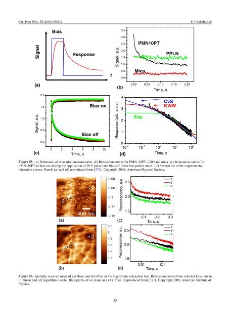
Rep. Prog. Phys. 73 (2010) 056502 S V Kalinin et al Signal (a) Signal, a.u. (c) 2.0 1.5 1.0 0.5 0.0 Bias Response Bias on Bias off 0 2 4 6 8 10 Time, s t Signal, a.u. Response (arb. units) (b) 3.5 3.0 2.5 2.0 1.5 1.0 0.5 0.0 4 3 2 1 0.00 0.05 0.10 0.15 0.20 Exp Time, s CvS KWW 0 10 -2 10 -1 10 0 10 1 10 2 (d) PMN10PT Mica Time, s PPLN Figure 55. (a) Schematic of relaxation measurement. (b) Relaxation curves for PMN–10PT, LNO and mica. (c) Relaxation curves for PMN–10PT in bias-on (during the application of 10 V pulse) and bias-off (after bias pulse) states. (d) Several fits of the experimental relaxation curves. Panels (a) and (d) reproduced from [372]. Copyright 2009, American Physical Society. 3 (a) 1 2 400 nm Piezoresponse, a.u. (c) 2.5 2.0 1.5 1 2 3 0.1 0.2 0.3 Time, s 3 (b) 1 2 Piezoresponse, a.u. (d) 2.5 2.0 1.5 0.01 0.1 Time, s 1 2 3 Figure 56. Spatially resolved maps of (a) slope and (b) offset in the logarithmic relaxation law. Relaxation curves from selected locations in (c) linear and (d) logarithmic scale. Histograms of (e) slope and (f ) offset. Reproduced from [371]. Copyright 2009, American Institute of Physics. 55
Rep. Prog. Phys. 73 (2010) 056502 field. It involves a complex coupling of long-range electromechanical interactions in a highly inhomogeneous and nonequilibrium system. Analytical solutions for the spatial and temporal distributions of polarization, electric field and stress during switching under PFM are generally not possible although semi-analytical solutions for the polarization distributions corresponding to the critical states or stable states have been attempted, as summarized in sections 3 and 4. To better understand the polarization switching mechanisms in PFM, a number of efforts to model the polarization evolution process using the phase-field method [65, 263, 295, 350, 388, 389] have been attempted. One of the main advantages for the phase-field method is the fact that one is able to model the temporal/spatial evolution of arbitrary domain morphologies under an applied electric field without explicitly tracking the positions of domain walls. Secondly, the inhomogeneous electric field and stress field distributions accompanying the polarization switching are readily available. Furthermore, the effect of structural defects such as grain boundaries, surfaces, dislocations and random defects can be incorporated without significantly increasing the computational time. Phase-field models have previously been applied to domain evolution during ferroelectric phase transitions and domain switching, effect of random defects and dislocations, as well as strain effect on transition temperatures and domain structures in thin films [390]. 5.1. Phase-field method During polarization switching the polarization distribution is always inhomogeneous, i.e. it depends on the spatial positions. In the phase-field approach, one employs the spatial distribution of local spontaneous polarization P (x) = (P 1 (x), P 2 (x), P 3 (x)) to describe a domain structure. Using the free energy for the unpolarized and unstrained crystal as the reference, the local free energy density as a function of strain and polarization using the Landau–Devonshire theory of ferroelectrics is f bulk (ε(x), P (x)) = 1 2 α ij P i (x) P j (x) + 1 4 γ ij klP i (x) P j (x) P k (x)P l (x) + 1 6 ω ij klmnP i (x)P j (x) P k (x)P l (x)P m (x)P n (x) + ··· 1 2 c ij klε ij (x) ε kl (x) − 1 2 q ij klε ij (x)P k (x)P l (x), (5.1) where α ij , γ ij kl and ω ij klmn are the phenomenological Landau expansion coefficients and c ij kl and q ij kl are the elastic and electrostrictive constant tensors, respectively. All the coefficients are generally assumed to be constant except α ij which is linearly proportional to temperature, i.e. α ij = αij o (T − T o), where T o is the Curie temperature. It should be noted that the coefficients in equation (5.1) correspond to zero strain while experiments are usually conducted at zero stress. In order to use the materials constants and Landau coefficients from stress-free conditions, we rewrite the free energy for zero stress. One first obtains the spontaneous strain, i.e. the strain or crystal deformation at zero stress, ε o ij (P k) = 1 2 s ij mnq mnkl P k P l = Q ij kl P k P l , (5.2) S V Kalinin et al where Q ij kl are the electrostrictive coefficients measured experimentally. Substituting the spontaneous strain from equation (5.2) for the strain in equation (5.1), we have the free energy at zero stress as g bulk (P(x)) = 1 2 α ij P i (x)P j (x) + 1 4 γ ij ′ kl P i(x)P j (x)P k (x) P l (x) + 1 6 ω ij klmnP i (x)P j (x) P k (x)P l (x)P m (x)P n (x) + ···, (5.3) where the α ij and ω ij klmn remain the same for zero stress as for zero strain, but γ ij kl at constant strain is changed to γ ij ′ kl at zero stress with γ ′ ij kl = γ ij kl − 2c mnop Q mnij Q opkl . (5.4) The free energy at zero strain and that at zero stress are related by f bulk ( εij (x), P (x) ) = g bulk (P(x)) + f elast ( Pi (x) ,ε ij (x) ) , where ( f elast P(x), εij (x) ) = 1 2 c ( ij kl εij (x) − εij o (x)) × ( ε kl (x) − εkl o (x)) . (5.5) For a domain structure, the electrostatic energy contains contributions from an external applied field E ex , the energy due to inhomogeneous polarization distribution δP i (x) = P i (x)− P¯ i and the depolarization energy F dep if the crystal is finite and the surface polarization charge is not fully compensated: ∫ ∫ F elec = V − 1 2 f elec (P i (x), E i (x)) dV =− P i (x) Ei ex (x)dV V ∫ ( ) E i (x)δP j (x)dV + F dep P ¯i , (5.6) V where P¯ i is the average polarization and E i is the ith component of the electric field generated by the heterogeneous polarization distribution δP i (x). The total free energy of an inhomogeneous domain structure is given by Ginzburg–Landau free energy functional: ∫ F = [f bulk (P i ) + f grad (∂P i /∂x j ) + f elast (P i ,ε ij ) V + f elec (P i ,E i )]d 3 x (5.7) in which f bulk is the bulk free energy density, f grad is the gradient energy that is only nonzero around domain walls and other interfaces where the polarization is inhomogeneous, f grad = 1 2 G ij klP i,j P k,l , (5.8) where P i,j = ∂P i /∂x j and G ij kl is the gradient energy coefficient. To obtain the elastic strain energy density f elast in equation (5.5), one needs to solve the mechanical equilibrium equation for a given domain structure. For a bulk single crystal with periodic boundary conditions, one can use Khachaturyan’s elasticity theory [391, 392]. For thin films, the mechanical boundary conditions become more complicated. The top surface is stress-free and the bottom surface is constrained by the substrate. As it has been shown in [393, 394], the solution to the mechanical equilibrium equations for 56
Page 1 and 2:
Home Search Collections Journals Ab
Page 3 and 4:
Rep. Prog. Phys. 73 (2010) 056502 S
Page 5 and 6: Rep. Prog. Phys. 73 (2010) 056502 S
Page 15 and 16: Rep. Prog. Phys. 73 (2010) 056502 i
Page 31 and 32: Rep. Prog. Phys. 73 (2010) 056502 F
Page 33 and 34: Rep. Prog. Phys. 73 (2010) 056502
Page 37 and 38: Rep. Prog. Phys. 73 (2010) 056502 a
Page 49 and 50: Rep. Prog. Phys. 73 (2010) 056502 D
Page 51 and 52: Rep. Prog. Phys. 73 (2010) 056502 (
Page 55: Rep. Prog. Phys. 73 (2010) 056502 S
Page 61 and 62: Rep. Prog. Phys. 73 (2010) 056502 d
Page 63 and 64: Rep. Prog. Phys. 73 (2010) 056502 W
Page 65 and 66: Rep. Prog. Phys. 73 (2010) 056502 [
Page 67 and 68: Rep. Prog. Phys. 73 (2010) 056502 [
show all

Local polarization dynamics in ferroelectric materials

Create successful ePaper yourself

Delete template?

Save as template?