Local polarization dynamics in ferroelectric materials

Rep. Prog. Phys. 73 (2010) 056502
S V Kalinin et al
10 3 l
l
r
∆l
(a) LNO
Domains sizes (nm)
10 2
10
10 3 l l
10 2
r
10
∆l
(b) LTO
1
1 10 10 2 10 3 10 4
Applied bias V (V)
1
1 10 10 2 10 3 10 4
Applied bias V (V)
Domains sizes (nm)
10 2
10
1
10 3 l
l
r
(c) PTO
∆l
1 10 10 2 10 3 10 4
Applied bias V (V)
10 3 l l
r
10 2
10 ∆l
(d) PZT
1
1 10 10 2 10 3
Applied bias V (V)
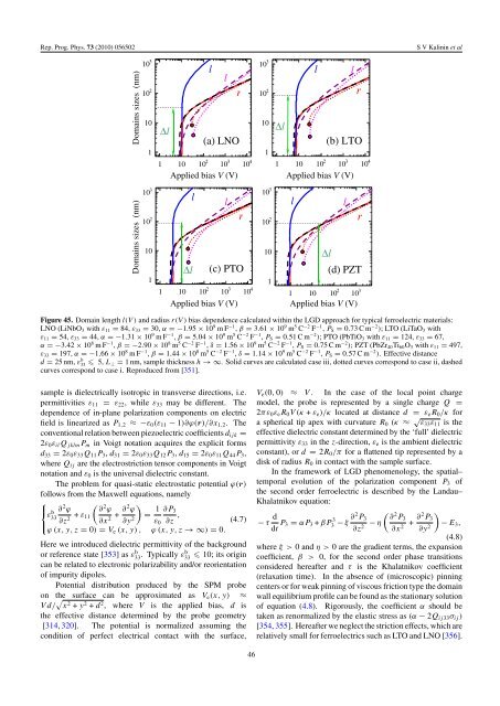
Figure 45. Domain length l(V ) and radius r(V) bias dependence calculated within the LGD approach for typical ferroelectric materials:
LNO (LiNbO 3 with ε 11 = 84, ε 33 = 30, α =−1.95 × 10 9 mF −1 , β = 3.61 × 10 9 m 5 C −2 F −1 , P S = 0.73Cm −2 ); LTO (LiTaO 3 with
ε 11 = 54, ε 33 = 44, α =−1.31 × 10 9 mF −1 , β = 5.04 × 10 9 m 5 C −2 F −1 , P S = 0.51Cm −2 ); PTO (PbTiO 3 with ε 11 = 124, ε 33 = 67,
α =−3.42 × 10 8 mF −1 , β =−2.90 × 10 8 m 5 C −2 F −1 , δ = 1.56 × 10 9 m 5 C −2 F −1 , P S = 0.75Cm −2 ); PZT (PbZr 40 Ti 60 O 3 with ε 11 = 497,
ε 33 = 197, α =−1.66 × 10 8 mF −1 , β = 1.44 × 10 8 m 5 C −2 F −1 , δ = 1.14 × 10 9 m 5 C −2 F −1 , P S = 0.57Cm −2 ). Effective distance
d = 25 nm, ε b 33 5, L ⊥ = 1 nm, sample thickness h →∞. Solid curves are calculated case iii, dotted curves correspond to case ii, dashed
curves correspond to case i. Reproduced from [351].
sample is dielectrically isotropic in transverse directions, i.e.
permittivities ε 11 = ε 22 , while ε 33 may be different. The
dependence of in-plane polarization components on electric
field is linearized as P 1,2 ≈−ε 0 (ε 11 − 1)∂ϕ(r)/∂x 1,2 . The
conventional relation between piezoelectric coefficients d ij k =
2ε 0 ε il Q jklm P m in Voigt notation acquires the explicit forms
d 33 = 2ε 0 ε 33 Q 11 P 3 , d 31 = 2ε 0 ε 33 Q 12 P 3 , d 15 = 2ε 0 ε 11 Q 44 P 3 ,
where Q ij are the electrostriction tensor components in Voigt
notation and ε 0 is the universal dielectric constant.
The problem for quasi-static electrostatic potential ϕ(r)
follows from the Maxwell equations, namely
⎧
⎨
ε b ∂ 2 (
ϕ ∂ 2 )
33
⎩
∂z + ε ϕ
2 11
∂x + ∂2 ϕ
= 1 ∂P 3
2 ∂y 2 ε 0 ∂z ,
(4.7)
ϕ (x,y,z = 0) = V e (x,y) , ϕ(x,y,z →∞) = 0.
Here we introduced dielectric permittivity of the background
or reference state [353] asε33 b . Typically εb 33
10; its origin
can be related to electronic polarizability and/or reorientation
of impurity dipoles.
Potential distribution produced by the SPM probe
on the surface can be approximated as V e (x, y) ≈
Vd/ √ x 2 + y 2 + d 2 , where V is the applied bias, d is
the effective distance determined by the probe geometry
[314, 320]. The potential is normalized assuming the
condition of perfect electrical contact with the surface,
V e (0, 0) ≈ V . In the case of the local point charge
model, the probe is represented by a single charge Q =
2πε 0 ε e R 0 V(κ+ ε e )/κ located at distance d = ε e R 0 /κ for
a spherical tip apex with curvature R 0 (κ ≈ √ ε 33 ε 11 is the
effective dielectric constant determined by the ‘full’ dielectric
permittivity ε 33 in the z-direction, ε e is the ambient dielectric
constant), or d = 2R 0 /π for a flattened tip represented by a
disk of radius R 0 in contact with the sample surface.
In the framework of LGD phenomenology, the spatial–
temporal evolution of the polarization component P 3 of
the second order ferroelectric is described by the Landau–
Khalatnikov equation:
− τ d (
dt P 3 = αP 3 + βP3 3 − ξ ∂2 P 3 ∂ 2 )
∂z − η P 3
2 ∂x + ∂2 P 3
− E 2 ∂y 2 3 ,
(4.8)
where ξ>0 and η>0 are the gradient terms, the expansion
coefficient, β > 0, for the second order phase transitions
considered hereafter and τ is the Khalatnikov coefficient
(relaxation time). In the absence of (microscopic) pinning
centers or for weak pinning of viscous friction type the domain
wall equilibrium profile can be found as the stationary solution
of equation (4.8). Rigorously, the coefficient α should be
taken as renormalized by the elastic stress as (α − 2Q ij 33 σ ij )
[354, 355]. Hereafter we neglect the striction effects, which are
relatively small for ferroelectrics such as LTO and LNO [356].
46