Local polarization dynamics in ferroelectric materials

Rep. Prog. Phys. 73 (2010) 056502
S V Kalinin et al
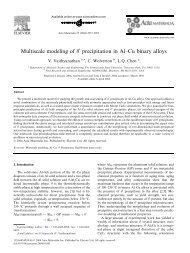
Figure 52. (a) Surface topography, (b) PFM amplitude and (c) PFM phase of an epitaxial PZT film. (d) Qualitative random field (RF) and
random bond (RB) disorder map. The RF disorder is defined as (|PNB|−|NNB|)/2, the RB disorder is defined as (|PNB| + |NNB|)/2.
Hysteresis loops illustrating the effect of (e) RF and (f ) RB disorder on the loop shape (comp. figure 1). Reproduced from [65]. Copyright
2008, Nature Publishing Group.
points, yielding the 3D PR(x,y,t) data arrays, where PR
is the piezoresponse signal, (x, y) is the coordinate and t
is the time. An analysis of the resulting PR(x,y,t) using
functional fit P R(t) = f (α, t), where α = α 1 ,...,α n is
an n-dimensional parameter vector, allows maps of α i (x, y)
describing the spatial variability of relaxation behavior to
be constructed. As an example, the fit using the stretched
exponential law, P R(t) = A 0 + A 1 exp(−(t/τ) β ) with n = 4
yields spatially resolved maps of relaxing, A 1 , and nonrelaxing,
A 0 , polarization components, relaxation time, τ, and
exponent, β (not shown). Alternatively, the fitting can be
performed using power law or logarithmic function.
The TR-PFM data were fitted using a logarithmic function
and the resulting spatial maps of offset, B 0 (x, y), and slope,
B 1 (x, y), are shown in figures 56(a) and (b). A number
Figure 53. Hysteresis loop with the corresponding domain images.
Reproduced from [366]. Copyright 2008, American Institute of
Physics.
4.5.2. Spatially resolved time spectroscopy imaging. The
single point TR-PFS can be extended to a mapping method
to explore spatial variability of relaxation behavior. The
measurements are performed on a densely spaced grid of
53
of relaxation curves extracted from regions of dissimilar
contrast in figure 56(a), (b) are shown in figures 56(c) and
(d). Note that relaxation behavior varies between adjacent
locations, illustrating the presence of mesoscopic dynamic
inhomogeneity on the ergodic relaxor surface. The slope
distribution is relatively narrow, B 1 =−0.10±0.02 within the
image, and close to Gaussian. In comparison, the distribution
of offsets is broader, B 1 = −1.5 ± 0.5, and is strongly