Local polarization dynamics in ferroelectric materials

Rep. Prog. Phys. 73 (2010) 056502
a film–substrate system can be obtained by combining
Khachaturyan’s mesoscopic elasticity theory [391, 392] and
the Stroh formalism of anisotropic elasticity [395]. In
obtaining the elastic energy, the local distributions of
mechanical displacements, strain and stress are also readily
available for a given domain structure and external boundary
conditions.
Similarly, the electrical energy density, f elec , in equation
(5.6) can be obtained by solving the electrostatic equation. For
the simple case that the depolarization field is compensated and
the external field is uniform, we have the electrostatic energy
for a single crystal,
∫
V
f elec d 3 V = 1 2
∫ ∣ ∣ n i P o
i (g)∣ ∣ 2
n j κ jk n k
d 3 g
(2π) 3 − ( Ei
ex )
P¯
i V, (5.9)
where Pk o(g) = ∫ V P k o(x)e−ig·x d 3 x, κ jk is the dielectric
constant tensor and n i is the ith component of unit vector,
g i /|g|. In equation (5.9), the reciprocal space origin, g = 0,
is excluded in the integration. Equation (5.9) shows the
dependence of electrostatic energy on dielectric constants, the
domain structure and the external applied field. For electric
boundary conditions that are inhomogeneous at the boundary,
e.g. under PFM, the electrostatic equilibrium equation is solved
using a specified inhomogeneous boundary condition for the
electric potential, φ,
φ substrate−film interface = 0,φ film surface = φ 1 (x 1 ,x 2 ) (5.10)
using the same strategy as the elastic solution for thin films
[396].
With all the important energetic contributions to the total
free energy, the temporal evolution of the polarization vector
field, and thus the domain structure, is then described by the
time-dependent Ginzburg–Landau (TDGL) equations,
∂P i (x,t)
∂t
δF
=−L
δP i (x,t) , (5.11)
where L is the kinetic coefficient related to the domainwall
mobility. For a given initial distribution of polarization,
numerical solution to equation (5.11) yields the temporal and
spatial evolution of polarization, and thus domain switching
under an external field.
5.2. Modeling the electric potential distribution from PFM
To model the domain writing process by PFM, one needs
quantitative information on the electric potential or electric
field distribution produced by the probe. The actual
distribution will depend on the size and shape of the probe,
and its accurate determination is difficult and requires finiteelement-type
of calculations with the knowledge of precise
probe geometry. Most existing theories and numerical
simulations of ferroelectric domain switching under PFM
assumed point-charge-type of electric potential distributions.
For example, in phase-field simulations of domain switching
under PFM, the tip-induced electric potential distribution on a
S V Kalinin et al
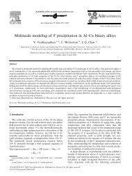
Figure 57. Variation of nucleation voltage as a function of effective
tip size.
sample surface is approximated by a two-dimensional Lorentzlike
function [350, 388],
[
]
γ 2
φ 1 (x 1 ,x 2 ) = φ 0 ( )
x1 − x1
0 2 ( )
+ x2 − x2
0 2
, (5.12)
+ γ
2
where x 1 and x 2 are the coordinates on the surface, (x 0 1 ,x0 2 ) is
the location of the tip (the peak of distribution) and γ is the
distance from the tip over which the applied electric potential
reduces to half of its peak value, φ 0 .
5.3. Nucleation bias
The nucleation bias is defined as the minimum applied
electric potential required to nucleate a new domain under
PFM. To determine the nucleation bias of a new domain
in a phase-field simulation, one starts with a single crystal
single ferroelectric domain state and impose an electric
potential distribution according to equation (5.12) as the
electric boundary conditions. One then gradually increases
the potential value φ 0 with small intervals. The minimum
potential value at which a new domain appears under PFM
is determined as the nucleation bias. However, it should be
noted that the nucleation bias is strongly sensitive to the probe
geometry, or in our simple potential model, to the parameter γ .
As an example, the dependence of nucleation bias on γ was
demonstrated using a BiFeO 3 epitaxial thin film consisting
of a single rhombohedral domain with polarization direction
along [¯1 ¯1 1] [1]. To find the critical nucleation potential, the
potential φ 0 was slowly increased in increment of 0.05 V. At
a sufficiently high value of φ 0 , a new rhombohedral domain
with polarization along [¯1 ¯1 ¯1] was found to nucleate below the
tip, and the corresponding value for φ 0 was identified as the
nucleation potential. The nucleation bias as a function of γ is
shown in figure 57. For the ranges of tip parameters consistent
with the measured domain wall width, the nucleation bias is
∼4.8 ± 0.5V.
Since there are no defects or thermal fluctuations
considered in the model, the nucleation bias in a phase-field
57