Local polarization dynamics in ferroelectric materials

Rep. Prog. Phys. 73 (2010) 056502
S V Kalinin et al
Figure 14. (a) Schematics of a PFM measurement across a 180 ◦ domain wall. (b) Piezoresponse calculation from cylindrical domain.
Reproduced from [186]. Copyright 2007, American Institute of Physics.
(pm/V)
d 33
eff
75 3
50
25
1
2
4
(a)
0
-25
-50
-75
-2 -1 0 1 2
(a-a 0 )/R 0
(pm/V)
d 35
eff
30
20
10
0
(d)
3
2
4
1
-10
-20
-4 -2 0 2 4
(a-a 0 )/R 0
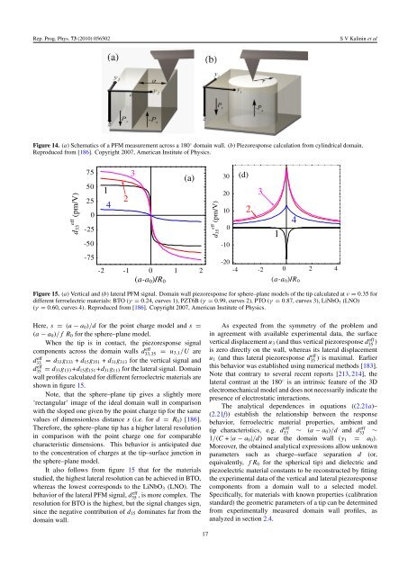
Figure 15. (a) Vertical and (b) lateral PFM signal. Domain wall piezoresponse for sphere–plane models of the tip calculated at ν = 0.35 for
different ferroelectric materials: BTO (γ = 0.24, curves 1), PZT6B (γ = 0.99, curves 2), PTO (γ = 0.87, curves 3), LiNbO 3 (LNO)
(γ = 0.60, curves 4). Reproduced from [186]. Copyright 2007, American Institute of Physics.
Here, s = (a − a 0 )/d for the point charge model and s =
(a − a 0 )/f R 0 for the sphere–plane model.
When the tip is in contact, the piezoresponse signal
components across the domain walls d33,35 eff = u 3,1/U are
d33 eff = d 33g 333 + d 15 g 351 + d 31 g 313 for the vertical signal and
d35 eff = d 33g 133 +d 15 g 151 +d 31 g 113 for the lateral signal. Domain
wall profiles calculated for different ferroelectric materials are
shown in figure 15.
Note, that the sphere–plane tip gives a slightly more
‘rectangular’ image of the ideal domain wall in comparison
with the sloped one given by the point charge tip for the same
values of dimensionless distance s (i.e. for d = R 0 ) [186].
Therefore, the sphere–plane tip has a higher lateral resolution
in comparison with the point charge one for comparable
characteristic dimensions. This behavior is anticipated due
to the concentration of charges at the tip–surface junction in
the sphere–plane model.
It also follows from figure 15 that for the materials
studied, the highest lateral resolution can be achieved in BTO,
whereas the lowest corresponds to the LiNbO 3 (LNO). The
behavior of the lateral PFM signal, d35 eff , is more complex. The
resolution for BTO is the highest, but the signal changes sign,
since the negative contribution of d 15 dominates far from the
domain wall.
As expected from the symmetry of the problem and
in agreement with available experimental data, the surface
vertical displacement u 3 (and thus vertical piezoresponse d35 eff)
is zero directly on the wall, whereas its lateral displacement
u 1 (and thus lateral piezoresponse d35 eff ) is maximal. Earlier
this behavior was established using numerical methods [183].
Note that contrary to several recent reports [213, 214], the
lateral contrast at the 180 ◦ is an intrinsic feature of the 3D
electromechanical model and does not necessarily indicate the
presence of electrostatic interactions.
The analytical dependences in equations ((2.21a)–
(2.21f)) establish the relationship between the response
behavior, ferroelectric material properties, ambient and
tip characteristics, e.g. d33 eff ∼ (a − a 0 )/d and d eff
33
∼
1/(C + |a − a 0 |/d) near the domain wall (y 1 = a 0 ).
Moreover, the obtained analytical expressions allow unknown
parameters such as charge–surface separation d (or,
equivalently, fR 0 for the spherical tip) and dielectric and
piezoelectric material constants to be reconstructed by fitting
the experimental data of the vertical and lateral piezoresponse
components from a domain wall to a selected model.
Specifically, for materials with known properties (calibration
standard) the geometric parameters of a tip can be determined
from experimentally measured domain wall profiles,
analyzed in section 2.4.
as
17