STATE OF THE CLIMATE IN 2009

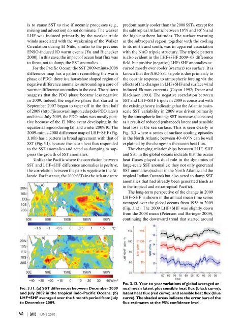
is to cause SST to rise if oceanic processes (e.g.,mixing and advection) do not dominate. The weakerLHF was induced primarily by the weaker tradewinds associated with the weakening of the WalkerCirculation during El Niño, similar to the previousENSO-induced IO warm events (Yu and Rienecker2000). In this case, the impact of ocean heat flux wasto force, not to damp, the SST anomalies.For the Pacific Ocean, the SST 2009-minus-2008difference map has a pattern resembling the warmphase of PDO: there is a horseshoe shaped region ofnegative difference anomalies surrounding a core ofwarmer difference anomalies to the east. The patternsuggests that the PDO phase became less negativein 2009. Indeed, the negative phase that started inSeptember 2007 began to taper off in the first halfof 2009 (http://jisao.washington.edu/pdo/PDO.latest)and since July 2009, the PDO index was mostly positivebecause of the El Niño event developing in theequatorial region during fall and winter 2009/10. The2009-minus-2008 difference map of LHF+SHF (Fig.3.10b) has a pattern in broad agreement with that ofSST (Fig. 3.1), because the ocean heat flux respondedto the SST anomalies and acted as damping to suppressthe growth of SST anomalies.Unlike the Pacific where the correlation betweenSST and LHF+SHF difference anomalies is positive,the correlation between the pair is negative in the Atlantic.For instance, the 2009 SSTs in the Atlantic werepredominantly cooler than the 2008 SSTs, except forthe subtropical Atlantic between 15°N and 30°N andthe high-northern latitudes. The surface warmingin the subtropical region, together with the coolingto its north and south, was in apparent associationwith the NAO tripole structure. The tripole patternis also evident in the LHF+SHF 2009–08 differencefield, but positive (negative) LHF+SHF anomalies occurredmostly over cooler (warmer) sea surface. It isknown that the NAO SST tripole is due primarily tothe oceanic response to atmospheric forcing via theeffects of the changes in LHF+SHF and surface windinduced Ekman currents (Cayan 1992; Deser andBlackmon 1993). The negative correlation betweenSST and LHF+SHF tripole in 2009 is consistent withthe existing theory, indicating that the Atlantic basinscaleSST variability in 2009 was driven primarilyby the atmospheric forcing: SST increases (decreases)as a result of reduced (enhanced) latent and sensibleheat loss at the sea surface. This is seen clearly inFig. 3.3 where a series of surface cooling episodesin the North Atlantic between 40–60°N can be wellexplained by the changes in the ocean heat flux.The changing relationships between LHF+SHFand SST in the global oceans indicate that the oceanheat fluxes played a dual role in the dynamics oflarge-scale SST anomalies: they not only generatedSST anomalies (such as in the North Atlantic and thetropical Indian Oceans) but also acted to damp SSTanomalies that had already been generated (such asin the tropical and extratropical Pacific).The long-term perspective of the change in 2009LHF+SHF is shown in the annual mean time seriesaveraged over the global oceans from 1958 to 2009(Fig. 3.12). The 2009 LHF+SHF was slightly downfrom the 2008 mean (Peterson and Baringer 2009),continuing the downward trend that started aroundFig. 3.11. (a) SST differences between December 2009and July 2009 in the tropical Indo-Pacific Oceans. (b)LHF+SHF averaged over the 6 month period from Julyto December 2009.Fig. 3.12. Year-to-year variations of global averaged annualmean latent plus sensible heat flux (black curve),latent heat flux (red curve), and sensible heat flux (bluecurve). The shaded areas indicate the error bars of theflux estimates at the 95% confidence level.S62 | juNE 2010