STATE OF THE CLIMATE IN 2009

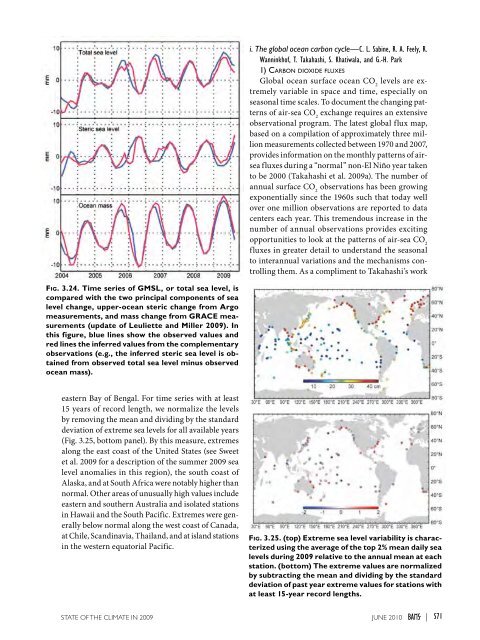
i. The global ocean carbon cycle—C. L. Sabine, R. A. Feely, R.Wanninkhof, T. Takahashi, S. Khatiwala, and G.-H. Park1) Carbon dioxide fluxesGlobal ocean surface ocean CO 2levels are extremelyvariable in space and time, especially onseasonal time scales. To document the changing patternsof air-sea CO 2exchange requires an extensiveobservational program. The latest global flux map,based on a compilation of approximately three millionmeasurements collected between 1970 and 2007,provides information on the monthly patterns of airseafluxes during a “normal” non-El Niño year takento be 2000 (Takahashi et al. 2009a). The number ofannual surface CO 2observations has been growingexponentially since the 1960s such that today wellover one million observations are reported to datacenters each year. This tremendous increase in thenumber of annual observations provides excitingopportunities to look at the patterns of air-sea CO 2fluxes in greater detail to understand the seasonalto interannual variations and the mechanisms controllingthem. As a compliment to Takahashi’s workFig. 3.24. Time series of GMSL, or total sea level, iscompared with the two principal components of sealevel change, upper-ocean steric change from Argomeasurements, and mass change from GRACE measurements(update of Leuliette and Miller 2009). Inthis figure, blue lines show the observed values andred lines the inferred values from the complementaryobservations (e.g., the inferred steric sea level is obtainedfrom observed total sea level minus observedocean mass).eastern Bay of Bengal. For time series with at least15 years of record length, we normalize the levelsby removing the mean and dividing by the standarddeviation of extreme sea levels for all available years(Fig. 3.25, bottom panel). By this measure, extremesalong the east coast of the United States (see Sweetet al. 2009 for a description of the summer 2009 sealevel anomalies in this region), the south coast ofAlaska, and at South Africa were notably higher thannormal. Other areas of unusually high values includeeastern and southern Australia and isolated stationsin Hawaii and the South Pacific. Extremes were generallybelow normal along the west coast of Canada,at Chile, Scandinavia, Thailand, and at island stationsin the western equatorial Pacific.Fig. 3.25. (top) Extreme sea level variability is characterizedusing the average of the top 2% mean daily sealevels during 2009 relative to the annual mean at eachstation. (bottom) The extreme values are normalizedby subtracting the mean and dividing by the standarddeviation of past year extreme values for stations withat least 15-year record lengths.STATE OF THE CLIMATE IN 2009 juNE 2010 |S71