- Page 2 and 3:
Lecture Notesin Control and Informa
- Page 4 and 5:
Series Advisory BoardF. Allgöwer,
- Page 7 and 8:
ContentsFoundations and History of
- Page 9 and 10:
ContentsIXRobustness, Robust Design
- Page 11 and 12:
ContentsXIHybrid NMPC Control of a
- Page 13 and 14:
Nonlinear Model Predictive Control:
- Page 15 and 16:
Nonlinear Model Predictive Control:
- Page 17 and 18:
Nonlinear Model Predictive Control:
- Page 19 and 20:
Nonlinear Model Predictive Control:
- Page 21 and 22:
Nonlinear Model Predictive Control:
- Page 23 and 24:
Nonlinear Model Predictive Control:
- Page 25 and 26:
Nonlinear Model Predictive Control:
- Page 27 and 28: Nonlinear Model Predictive Control:
- Page 29 and 30: Hybrid MPC: Open-Minded but Not Eas
- Page 31 and 32: Hybrid MPC: Open-Minded but Not Eas
- Page 34 and 35: 22 S.E. Tuna et al.this says that i
- Page 36 and 37: 24 S.E. Tuna et al.In particular, f
- Page 38 and 39: 26 S.E. Tuna et al.W N (f(x, ¯κ N
- Page 40 and 41: 28 S.E. Tuna et al.where ᾱ := max
- Page 42 and 43: 30 S.E. Tuna et al.21.521.5µ=51
- Page 44 and 45: 32 S.E. Tuna et al.obstacle and gra
- Page 46 and 47: 34 S.E. Tuna et al.[19] C. Prieur.
- Page 48 and 49: 36 É. Gyurkovics and A.M. Elaiw[8]
- Page 50 and 51: 38 É. Gyurkovics and A.M. ElaiwWe
- Page 52: 40 É. Gyurkovics and A.M. ElaiwWe
- Page 55 and 56: Conditions for MPC Based Stabilizat
- Page 57 and 58: Conditions for MPC Based Stabilizat
- Page 59 and 60: Conditions for MPC Based Stabilizat
- Page 61 and 62: A Computationally Efficient Schedul
- Page 63 and 64: A Computationally Efficient Schedul
- Page 65 and 66: A Computationally Efficient Schedul
- Page 67 and 68: A Computationally Efficient Schedul
- Page 69 and 70: A Computationally Efficient Schedul
- Page 71 and 72: A Computationally Efficient Schedul
- Page 73 and 74: A Computationally Efficient Schedul
- Page 75 and 76: The Potential of Interpolation for
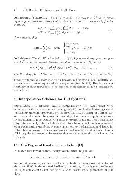
- Page 77: The Potential of Interpolation 65De
- Page 81 and 82: The Potential of Interpolation 693.
- Page 83 and 84: The Potential of Interpolation 71Pr
- Page 85 and 86: The Potential of Interpolation 73Th
- Page 87 and 88: The Potential of Interpolation 75de
- Page 89 and 90: Techniques for Uniting Lyapunov-Bas
- Page 91 and 92: Techniques for Uniting Lyapunov-Bas
- Page 93 and 94: Techniques for Uniting Lyapunov-Bas
- Page 95 and 96: Techniques for Uniting Lyapunov-Bas
- Page 97 and 98: Techniques for Uniting Lyapunov-Bas
- Page 99 and 100: Techniques for Uniting Lyapunov-Bas
- Page 101 and 102: Techniques for Uniting Lyapunov-Bas
- Page 103 and 104: Techniques for Uniting Lyapunov-Bas
- Page 105 and 106: 94 M. Lazar et al.Lipschitz continu
- Page 107 and 108: 96 M. Lazar et al.let X T ⊆ X den
- Page 109 and 110: 98 M. Lazar et al.S 0 {j ∈S|0
- Page 111 and 112: 100 M. Lazar et al.Fig. 1. State-sp
- Page 113 and 114: 102 M. Lazar et al.[11] Grimm, G.,
- Page 115 and 116: Model Predictive Control for Nonlin
- Page 117 and 118: Model Predictive Control for Nonlin
- Page 119 and 120: Model Predictive Control for Nonlin
- Page 121 and 122: Model Predictive Control for Nonlin
- Page 123 and 124: ReferencesModel Predictive Control
- Page 125 and 126: 116 F.A.C.C. Fontes, L. Magni, and
- Page 127 and 128: 118 F.A.C.C. Fontes, L. Magni, and
- Page 129 and 130:
120 F.A.C.C. Fontes, L. Magni, and
- Page 131 and 132:
122 F.A.C.C. Fontes, L. Magni, and
- Page 133 and 134:
124 F.A.C.C. Fontes, L. Magni, and
- Page 135 and 136:
126 F.A.C.C. Fontes, L. Magni, and
- Page 137 and 138:
128 F.A.C.C. Fontes, L. Magni, and
- Page 139 and 140:
On the Computation of Robust Contro
- Page 141 and 142:
On the Computation of Robust Contro
- Page 143 and 144:
On the Computation of Robust Contro
- Page 145 and 146:
On the Computation of Robust Contro
- Page 147 and 148:
On the Computation of Robust Contro
- Page 149 and 150:
142 M. Srinivasarao, S.C. Patwardha
- Page 151 and 152:
144 M. Srinivasarao, S.C. Patwardha
- Page 153 and 154:
146 M. Srinivasarao, S.C. Patwardha
- Page 155 and 156:
148 M. Srinivasarao, S.C. Patwardha
- Page 157 and 158:
Nonlinear Model Predictive Control:
- Page 159 and 160:
Nonlinear Model Predictive Control:
- Page 161 and 162:
Nonlinear Model Predictive Control:
- Page 163 and 164:
Nonlinear Model Predictive Control:
- Page 165 and 166:
Nonlinear Model Predictive Control:
- Page 167 and 168:
Nonlinear Model Predictive Control:
- Page 169 and 170:
Numerical Methods for Efficient and
- Page 171 and 172:
Numerical Methods for Efficient and
- Page 173 and 174:
L i (s i ,u i ):=Numerical Methods
- Page 175 and 176:
Numerical Methods for Efficient and
- Page 177 and 178:
Numerical Methods for Efficient and
- Page 179 and 180:
Numerical Methods for Efficient and
- Page 181 and 182:
Numerical Methods for Efficient and
- Page 183 and 184:
Numerical Methods for Efficient and
- Page 185 and 186:
Numerical Methods for Efficient and
- Page 187 and 188:
182 A. Grancharova, T.A. Johansen,
- Page 189 and 190:
184 A. Grancharova, T.A. Johansen,
- Page 191 and 192:
186 A. Grancharova, T.A. Johansen,
- Page 193 and 194:
188 A. Grancharova, T.A. Johansen,
- Page 195 and 196:
190 A. Grancharova, T.A. Johansen,
- Page 197 and 198:
192 A. Grancharova, T.A. Johansen,
- Page 199 and 200:
194 V. Sakizlis et al.presented her
- Page 201 and 202:
196 V. Sakizlis et al.linear PWA fu
- Page 203 and 204:
198 V. Sakizlis et al.non-linear sy
- Page 205 and 206:
200 V. Sakizlis et al.Remark 1. For
- Page 207 and 208:
202 V. Sakizlis et al.One should no
- Page 209 and 210:
204 V. Sakizlis et al.g0.050.10.15x
- Page 211 and 212:
Interior-Point Algorithms for Nonli
- Page 213 and 214:
Interior-Point Algorithms for Nonli
- Page 215 and 216:
Interior-Point Algorithms for Nonli
- Page 217 and 218:
Interior-Point Algorithms for Nonli
- Page 219 and 220:
n p,2 ≤Interior-Point Algorithms
- Page 221 and 222:
Hard Constraints for Prioritized Ob
- Page 223 and 224:
Hard Constraints for Prioritized Ob
- Page 225 and 226:
Hard Constraints for Prioritized Ob
- Page 227 and 228:
Hard Constraints for Prioritized Ob
- Page 229 and 230:
Hard Constraints for Prioritized Ob
- Page 231 and 232:
Hard Constraints for Prioritized Ob
- Page 233 and 234:
A Nonlinear Model Predictive Contro
- Page 235 and 236:
A Nonlinear Model Predictive Contro
- Page 237 and 238:
A Nonlinear Model Predictive Contro
- Page 239 and 240:
A Nonlinear Model Predictive Contro
- Page 241 and 242:
A Nonlinear Model Predictive Contro
- Page 243 and 244:
Robustness and Robust Design of MPC
- Page 245 and 246:
Robustness and Robust Design of MPC
- Page 247 and 248:
Robustness and Robust Design of MPC
- Page 249 and 250:
Robustness and Robust Design of MPC
- Page 251 and 252:
Robustness and Robust Design of MPC
- Page 253 and 254:
Robustness and Robust Design of MPC
- Page 255 and 256:
Robustness and Robust Design of MPC
- Page 257 and 258:
Robustness and Robust Design of MPC
- Page 259 and 260:
MPC for Stochastic SystemsMark Cann
- Page 261 and 262:
y i (k) =∑n um=1MPC for Stochasti
- Page 263 and 264:
MPC for Stochastic Systems 259we ha
- Page 265 and 266:
MPC for Stochastic Systems 261form
- Page 267 and 268:
MPC for Stochastic Systems 263( )κ
- Page 269 and 270:
MPC for Stochastic Systems 265Fig.
- Page 271 and 272:
MPC for Stochastic Systems 267⎡
- Page 273 and 274:
NMPC for Complex Stochastic Systems
- Page 275 and 276:
NMPC for Complex Stochastic Systems
- Page 277 and 278:
NMPC for Complex Stochastic Systems
- Page 279 and 280:
NMPC for Complex Stochastic Systems
- Page 281 and 282:
NMPC for Complex Stochastic Systems
- Page 283 and 284:
NMPC for Complex Stochastic Systems
- Page 285 and 286:
NMPC for Complex Stochastic Systems
- Page 287 and 288:
284 H. Chen et al.of the moving hor
- Page 289 and 290:
286 H. Chen et al.Hence, at each sa
- Page 291 and 292:
288 H. Chen et al.control inputs in
- Page 293 and 294:
290 H. Chen et al.Corollary 1. The
- Page 295 and 296:
292 H. Chen et al.c A[mol/l]10−10
- Page 297 and 298:
294 H. Chen et al.[CSA97] H.Chen,C.
- Page 299 and 300:
296 L. Xie, P. Li, and G. Woznyand
- Page 301 and 302:
298 L. Xie, P. Li, and G. WoznyDeta
- Page 303 and 304:
300 L. Xie, P. Li, and G. Wozny3.2
- Page 305 and 306:
302 L. Xie, P. Li, and G. WoznyFig.
- Page 307 and 308:
304 L. Xie, P. Li, and G. Wozny[3]
- Page 309 and 310:
306 H. Arellano-Garcia et al.applic
- Page 311 and 312:
308 H. Arellano-Garcia et al.Fig. 1
- Page 313 and 314:
310 H. Arellano-Garcia et al.RECIPE
- Page 315 and 316:
312 H. Arellano-Garcia et al.optimi
- Page 317 and 318:
314 H. Arellano-Garcia et al.The re
- Page 319 and 320:
Interval Arithmetic in Robust Nonli
- Page 321 and 322:
Interval Arithmetic in Robust Nonli
- Page 323 and 324:
Interval Arithmetic in Robust Nonli
- Page 325 and 326:
Interval Arithmetic in Robust Nonli
- Page 327 and 328:
Interval Arithmetic in Robust Nonli
- Page 329 and 330:
Optimal Online Control of Dynamical
- Page 331 and 332:
Optimal Online Control of Dynamical
- Page 333 and 334:
Optimal Online Control of Dynamical
- Page 335 and 336:
Optimal Online Control of Dynamical
- Page 337 and 338:
State Estimation Analysed as Invers
- Page 339 and 340:
State Estimation Analysed as Invers
- Page 341 and 342:
State Estimation Analysed as Invers
- Page 343 and 344:
State Estimation Analysed as Invers
- Page 345 and 346:
State Estimation Analysed as Invers
- Page 347 and 348:
State Estimation Analysed as Invers
- Page 349 and 350:
Minimum-Distance Receding-Horizon S
- Page 351 and 352:
Minimum-Distance Receding-Horizon S
- Page 353 and 354:
Minimum-Distance Receding-Horizon S
- Page 355 and 356:
Minimum-Distance Receding-Horizon S
- Page 357 and 358:
Minimum-Distance Receding-Horizon S
- Page 359 and 360:
Minimum-Distance Receding-Horizon S
- Page 361 and 362:
New Extended Kalman Filter Algorith
- Page 363 and 364:
New Extended Kalman Filter Algorith
- Page 365 and 366:
New Extended Kalman Filter Algorith
- Page 367 and 368:
New Extended Kalman Filter Algorith
- Page 369 and 370:
NLMPC: A Platform for Optimal Contr
- Page 371 and 372:
NLMPC: A Platform for Optimal Contr
- Page 373 and 374:
NLMPC: A Platform for Optimal Contr
- Page 375 and 376:
NLMPC: A Platform for Optimal Contr
- Page 377 and 378:
NLMPC: A Platform for Optimal Contr
- Page 379 and 380:
NLMPC: A Platform for Optimal Contr
- Page 381 and 382:
NLMPC: A Platform for Optimal Contr
- Page 383 and 384:
NLMPC: A Platform for Optimal Contr
- Page 385 and 386:
384 K. Naidoo et al.polymer control
- Page 387 and 388:
386 K. Naidoo et al.are two key qua
- Page 389 and 390:
388 K. Naidoo et al.1. It greatly s
- Page 391 and 392:
390 K. Naidoo et al.However, with t
- Page 393 and 394:
392 K. Naidoo et al.Fig. 4. Bounded
- Page 395 and 396:
394 K. Naidoo et al.1. Maintain pro
- Page 397 and 398:
396 K. Naidoo et al.7 Commissioning
- Page 399 and 400:
398 K. Naidoo et al.[3] N.M.C. Oliv
- Page 401 and 402:
400 R. Franke and J. DoppelhamerImp
- Page 403 and 404:
402 R. Franke and J. DoppelhamerFig
- Page 405 and 406:
404 R. Franke and J. DoppelhamerFig
- Page 407 and 408:
406 R. Franke and J. Doppelhamer[3]
- Page 409 and 410:
408 B.A. Foss and T.S. Scheicritica
- Page 411 and 412:
410 B.A. Foss and T.S. ScheiFig. 2.
- Page 413 and 414:
412 B.A. Foss and T.S. Scheidiscuss
- Page 415 and 416:
414 B.A. Foss and T.S. ScheiOther a
- Page 417 and 418:
416 B.A. Foss and T.S. ScheiIn the
- Page 419 and 420:
Integration of Economical Optimizat
- Page 421 and 422:
Integration of Economical Optimizat
- Page 423 and 424:
Integration of Economical Optimizat
- Page 425 and 426:
Integration of Economical Optimizat
- Page 427 and 428:
Integration of Economical Optimizat
- Page 429 and 430:
Integration of Economical Optimizat
- Page 431 and 432:
Integration of Economical Optimizat
- Page 433 and 434:
Integration of Economical Optimizat
- Page 435 and 436:
Controlling Distributed Hyperbolic
- Page 437 and 438:
Controlling Distributed Hyperbolic
- Page 439 and 440:
Controlling Distributed Hyperbolic
- Page 441 and 442:
Controlling Distributed Hyperbolic
- Page 443 and 444:
444 K.R. Muske, A.E. Witmer, and R.
- Page 445 and 446:
446 K.R. Muske, A.E. Witmer, and R.
- Page 447 and 448:
448 K.R. Muske, A.E. Witmer, and R.
- Page 449 and 450:
450 K.R. Muske, A.E. Witmer, and R.
- Page 451 and 452:
452 K.R. Muske, A.E. Witmer, and R.
- Page 453 and 454:
Robust NMPC for a Benchmark Fed-Bat
- Page 455 and 456:
Robust NMPC for a Benchmark Fed-Bat
- Page 457 and 458:
Robust NMPC for a Benchmark Fed-Bat
- Page 459 and 460:
Robust NMPC for a Benchmark Fed-Bat
- Page 461 and 462:
Robust NMPC for a Benchmark Fed-Bat
- Page 463 and 464:
Real-Time Implementation of Nonline
- Page 465 and 466:
Real-Time Implementation of Nonline
- Page 467 and 468:
Real-Time Implementation of Nonline
- Page 469 and 470:
Real-Time Implementation of Nonline
- Page 471 and 472:
Non-linear Model Predictive Control
- Page 473 and 474:
NMPC of the Hashimoto Simulated Mov
- Page 475 and 476:
NMPC of the Hashimoto Simulated Mov
- Page 477 and 478:
NMPC of the Hashimoto Simulated Mov
- Page 479 and 480:
NMPC of the Hashimoto Simulated Mov
- Page 481 and 482:
NMPC of the Hashimoto Simulated Mov
- Page 483 and 484:
486 R. Lepore et al.In this study,
- Page 485 and 486:
488 R. Lepore et al.3 Control Strat
- Page 487 and 488:
490 R. Lepore et al.400.80.6|x−x
- Page 489 and 490:
492 R. Lepore et al.0.950.9w P;30.8
- Page 491 and 492:
Hybrid NMPC Control of a Sugar Hous
- Page 493 and 494:
Hybrid NMPC Control of a Sugar Hous
- Page 495 and 496:
Hybrid NMPC Control of a Sugar Hous
- Page 497 and 498:
Hybrid NMPC Control of a Sugar Hous
- Page 499 and 500:
Application of the NEPSAC Nonlinear
- Page 501 and 502:
Application of the NEPSAC Nonlinear
- Page 503 and 504:
Application of the NEPSAC Nonlinear
- Page 505 and 506:
Application of the NEPSAC Nonlinear
- Page 507 and 508:
Application of the NEPSAC Nonlinear
- Page 509 and 510:
Integrating Fault Diagnosis with No
- Page 511 and 512:
Integrating Fault Diagnosis with No
- Page 513 and 514:
Integrating Fault Diagnosis with No
- Page 515 and 516:
Integrating Fault Diagnosis with No
- Page 517 and 518:
Integrating Fault Diagnosis with No
- Page 519 and 520:
524 M. Alamirmin V (x u(·,x),T) un
- Page 521 and 522:
526 M. AlamirDefinition 4. The syst
- Page 523 and 524:
528 M. Alamir♭V is radially unbou
- Page 525 and 526:
530 M. AlamirBut according to the s
- Page 527 and 528:
532 M. AlamirFig. 2. Stabilization
- Page 529 and 530:
534 M. AlamirFig. 3. Closed loop be
- Page 531 and 532:
A New Real-Time Method for Nonlinea
- Page 533 and 534:
A New Real-Time Method for Nonlinea
- Page 535 and 536:
A New Real-Time Method for Nonlinea
- Page 537 and 538:
A New Real-Time Method for Nonlinea
- Page 539 and 540:
A New Real-Time Method for Nonlinea
- Page 541 and 542:
A New Real-Time Method for Nonlinea
- Page 543 and 544:
A New Real-Time Method for Nonlinea
- Page 545 and 546:
A Two-Time-Scale Control Scheme for
- Page 547 and 548:
A Two-Time-Scale Control Scheme for
- Page 549 and 550:
A Two-Time-Scale Control Scheme for
- Page 551 and 552:
A Two-Time-Scale Control Scheme for
- Page 553 and 554:
A Two-Time-Scale Control Scheme for
- Page 555 and 556:
A Two-Time-Scale Control Scheme for
- Page 557 and 558:
A Two-Time-Scale Control Scheme for
- Page 559 and 560:
566 X.-B. Hu and W.-H. Chen2 Online
- Page 561 and 562:
568 X.-B. Hu and W.-H. Chentime alo
- Page 563 and 564:
570 X.-B. Hu and W.-H. ChenFig. 3.
- Page 565 and 566:
572 X.-B. Hu and W.-H. ChenTable 4.
- Page 567 and 568:
574 M. Fujita et al. CameraCameraTa
- Page 569 and 570:
576 M. Fujita et al.J(u, t) =∫t+T
- Page 571 and 572:
578 M. Fujita et al.ξ 2[rad/s]6420
- Page 573 and 574:
580 M. Fujita et al.Acknowledgement
- Page 575 and 576:
582 A. Casavola, D. Famularo, and G
- Page 577 and 578:
584 A. Casavola, D. Famularo, and G
- Page 579 and 580:
4. c(t) ∈Cfor all t ∈ Z + ;5. T
- Page 581 and 582:
588 A. Casavola, D. Famularo, and G
- Page 583 and 584:
Distributed Model Predictive Contro
- Page 585 and 586:
Distributed Model Predictive Contro
- Page 587 and 588:
Distributed Model Predictive Contro
- Page 589 and 590:
Distributed Model Predictive Contro
- Page 591 and 592:
Distributed Model Predictive Contro
- Page 593 and 594:
Distributed Model Predictive Contro
- Page 595 and 596:
Distributed Model Predictive Contro
- Page 597 and 598:
Distributed Model Predictive Contro
- Page 599 and 600:
608 W.B. Dunbar and S. Desaand sequ
- Page 601 and 602:
610 W.B. Dunbar and S. Desademand r
- Page 603 and 604:
612 W.B. Dunbar and S. Desabacklog
- Page 605 and 606:
614 W.B. Dunbar and S. Desacasescas
- Page 607 and 608:
Robust Model Predictive Control for
- Page 609 and 610:
Robust Model Predictive Control for
- Page 611 and 612:
Robust Model Predictive Control for
- Page 613 and 614:
Robust Model Predictive Control for
- Page 615 and 616:
Robust Model Predictive Control for
- Page 617 and 618:
Robust Model Predictive Control for
- Page 619 and 620:
630 J.J. Arrieta-Camacho, L.T. Bieg
- Page 621 and 622:
632 J.J. Arrieta-Camacho, L.T. Bieg
- Page 623 and 624:
634 J.J. Arrieta-Camacho, L.T. Bieg
- Page 625 and 626:
636 J.J. Arrieta-Camacho, L.T. Bieg
- Page 627 and 628:
638 J.J. Arrieta-Camacho, L.T. Bieg
- Page 629 and 630:
Author IndexAlamir, Mazen 523Alamo,
- Page 631 and 632:
Lecture Notes in Control and Inform


![[Language - English] - Life Skills - Writing](https://img.yumpu.com/44143758/1/190x245/language-english-life-skills-writing.jpg?quality=85)