Violation in Mixing

More documents

Recommendations

Info

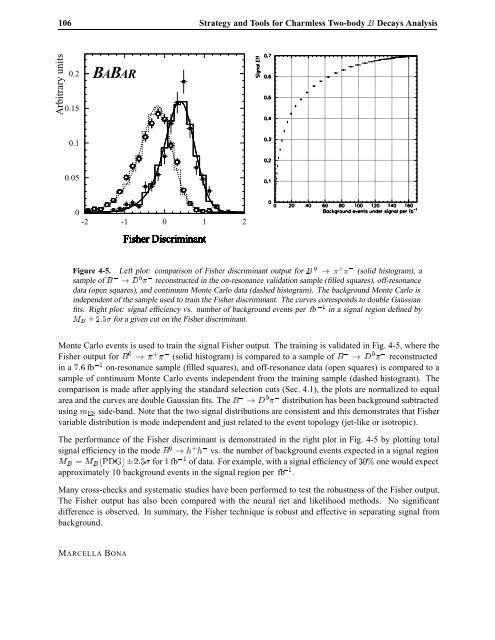
106 Strategy and Tools for Charmless Two-body � Decays Analysis Arbitrary units 0.2 0.15 0.1 0.05 BABAR 0 -2 -1 0 1 2 Fisher Discriminant Figure 4-5. Left plot: comparison of Fisher discriminant output for � � � � (solid histogram), a sample of � � � � reconstructed in the on-resonance validation sample (filled squares), off-resonance data (open squares), and continuum Monte Carlo data (dashed histogram). The background Monte Carlo is independent of the sample used to train the Fisher discriminant. The curves corresponds to double Gaussian fits. Right plot: signal efficiency vs. number of background events per fb Å� ¦ �� for a given cut on the Fisher discriminant. in a signal region defined by Monte Carlo events is used to train the signal Fisher output. The training is validated in Fig. 4-5, where the Fisher output for � � � � (solid histogram) is compared to a sample of � � � � reconstructed in a �� fb on-resonance sample (filled squares), and off-resonance data (open squares) is compared to a sample of continuum Monte Carlo events independent from the training sample (dashed histogram). The comparison is made after applying the standard selection cuts (Sec. 4.1), the plots are normalized to equal area and the curves are double Gaussian fits. The � � � � distribution has been background subtracted using Ñ�Ë side-band. Note that the two signal distributions are consistent and this demonstrates that Fisher variable distribution is mode independent and just related to the event topology (jet-like or isotropic). The performance of the Fisher discriminant is demonstrated in the right plot in Fig. 4-5 by plotting total signal efficiency in the mode � � � � vs. the number of background events expected in a signal region Å� � Å� È�� ¦ �� for fb of data. For example, with a signal efficiency of one would expect approximately 10 background events in the signal region per fb . Many cross-checks and systematic studies have been performed to test the robustness of the Fisher output. The Fisher output has also been compared with the neural net and likelihood methods. No significant difference is observed. In summary, the Fisher technique is robust and effective in separating signal from background. MARCELLA BONA
4.4 PID selection 107 In the case of the global maximum likelihood fit (see Sec. 4.6), no cuts are applied to the Fisher discriminant. Instead, signal-background discrimination is achieved by using � in the fit itself. Comparison of � for signal and background events is described in detail in section 4.6.1. In case of the counting analysis, a cut on the Fisher discriminant output is applied and it is chosen in order to optimize the statistical significance Ë � Ë � , where Ë and � are the number of expected signal and background events, respectively. After this cut, one should check that side-band background shape is wellmodeled by the ARGUS function fitted before applying these cuts, giving confidence that the same function can be used (see Sec. 4.6). 4.4 PID selection The difference between a Ã or a � in the final state taken here into account is apparent only in the reconstructed ¡�, for which there is a separation of less than �. The particle identification capabilities of the BABAR detector provide additional means to distinguish the two decays. Of primary importance is the �ÁÊ� information since the momenta of the two daughter tracks in these decays are in a region where the mean ��À ��Ü for kaons and pions differ by only about �. In principle, the �ÁÊ� can provide better than � separation of pions and kaons throughout the momentum region of the daughter tracks. The maximum likelihood fit makes direct use of the � ��Ö�Ò�ÓÚ angle, � , reconstructed by the �ÁÊ�. Each track is assigned a likelihood to be a pion or kaon based on the value of the reconstructed �. As a cross check, a second complementary method is pursued. It employs particle selector algorithms which provide lists of kaon and pion tracks that are used to separately identify the different final state modes. A cut on the number of signal photons observed in the �ÁÊ� is used to improve the � resolution and reduce the size of non-Gaussian tails. The cut Æ×�� is used, where Æ×�� is the number of observed signal photons for the track. Protons are explicitly removed with the cut � � Ô � ÑÖ��, where � Ô is the expected mean value of � for a proton of a given momentum. Electrons are removed by rejecting tracks which pass a tight selector criteria. The performance of the PID cuts are studied in the actual data using a pure sample of kaons and pions obtained from a control sample of � £ � � � , with � � Ã � . 4.4.1 � � £ � control sample In order to assess and parameterize the performance of the particle ID methods, without relying on Monte Carlo simulation, one must identify a source of pions and kaons, the selection of which does not utilize particle ID from the �ÁÊ�. An ideal control sample consists of the daughter tracks from � � Ã � decays in the reaction � £ � � � � Ã � � . The � (Ã) track is always the one with the same (opposite) charge as the � £ and cutting on the small � £ � mass difference ensures that there is virtually no contamination from incorrectly reconstructed � candidates (i.e. a true � � Ã � reconstructed as a � � � Ã candidate and then combined with a random track to form a � £ STRATEGY AND TOOLS FOR CHARMLESS TWO-BODY � DECAYS ANALYSIS
Page 1 and 2:
ÍÒ�Ú�Ö×�Ø��
Page 3 and 4:
Contents Introduction . ...........
Page 5 and 6:
4 Strategy and Tools for Charmless
Page 7 and 8:
7.2 Branching fraction � � �
Page 9 and 10:
Introduction The main goal of the B
Page 11 and 12:
1 �È Violation in the �� Sys
Page 13 and 14:
1.2 Neutral � Mesons 7 Note, howe
Page 15 and 16:
1.2 Neutral � Mesons 9 Applying t
Page 17 and 18:
1.2 Neutral � Mesons 11 �È �
Page 19 and 20:
1.2 Neutral � Mesons 13 ��
Page 21 and 22:
1.2 Neutral � Mesons 15 � ¡�
Page 23 and 24:
1.2 Neutral � Mesons 17 and � a
Page 25 and 26:
1.2 Neutral � Mesons 19 given tim
Page 27 and 28:
1.3 The Three Types of �È Violat
Page 29 and 30:
Page 31 and 32:
Page 33 and 34:
1.4 �È Violation in the Standard
Page 35 and 36:
Page 37 and 38:
Page 39 and 40:
Page 41 and 42:
Page 43 and 44:
1.5 Determination of « 37 1.5 Dete
Page 45 and 46:
1.5 Determination of « 39 Assuming
Page 47 and 48:
1.5 Determination of « 41 Figure 1
Page 49 and 50:
1.5 Determination of « 43 b q (a)
Page 51 and 52:
1.5 Determination of « 45 � �
Page 53 and 54:
2 The BABAR Experiment 2.1 Physics
Page 55 and 56:
2.1 Physics at � � B Factory op
Page 57 and 58:
2.2 The BABAR detector. 51 Integrat
Page 59 and 60:
2.2 The BABAR detector. 53 The dete
Page 61 and 62: 2.2 The BABAR detector. 55 two oute
Page 63 and 64: 2.2 The BABAR detector. 57 SVT Effi
Page 65 and 66: 2.2 The BABAR detector. 59 324 1015
Page 67 and 68: Efficiency 2.2 The BABAR detector.
Page 69 and 70: 2.2 The BABAR detector. 63 2.2.4 Th
Page 71 and 72: entries per mrad 2.2 The BABAR dete
Page 73 and 74: 2.2 The BABAR detector. 67 entries
Page 75 and 76: 2.2 The BABAR detector. 69 energies
Page 77 and 78: 2.2 The BABAR detector. 71 The main
Page 79 and 80: Efficiency 2.2 The BABAR detector.
Page 81 and 82: 2.2 The BABAR detector. 75 Table 2-
Page 83 and 84: 3 Ã Ë reconstruction and efficien
Page 85 and 86: 3.3 Studies on data 79 19.5° BINS
Page 87 and 88: 3.3 Studies on data 81 ¯ off-reson
Page 89 and 90: 3.3 Studies on data 83 0.504 0.502
Page 91 and 92: 3.3 Studies on data 85 0.03 0.025 0
Page 95 and 96: 3.3 Studies on data 89 N(π + π -
Page 99 and 100: 3.3 Studies on data 93 Figure 3-13.
Page 103 and 104: 4 Strategy and Tools for Charmless
Page 105 and 106: 4.2 Event selection 99 channel sele
Page 107 and 108: 4.2 Event selection 101 ÀÐ �
Page 109 and 110: 4.2 Event selection 103 Figure 4-2.
Page 111: 4.3 Background fighting 105 Figure
Page 115 and 116: 4.4 PID selection 109 θ c Cut Effi
Page 117 and 118: 4.5 Tracking Corrections 111 Ë�
Page 119 and 120: 4.6 Analysis methods 113 Ñ�Ë si
Page 121 and 122: 4.6 Analysis methods 115 Events/2.5
Page 123 and 124: 4.6 Analysis methods 117 Figure 4-1
Page 125 and 126: 4.6 Analysis methods 119 θ c radia
Page 127 and 128: 5 Measurement of Branching Fraction
Page 129 and 130: 5.2 Ã Ë reconstruction 123 1 0.8
Page 131 and 132: 5.3 Analysis Strategy 125 0.35 0.3
Page 133 and 134: 5.4 Background Suppression and PDF
Page 139 and 140: 5.5 Maximum likelihood analysis 133
Page 151 and 152: 5.6 Counting analysis 145 Table 5-1
Page 153 and 154: 5.7 Determination of branching frac
Page 155 and 156: 6 Measurement of Branching Fraction
Page 157 and 158: 6.3 The maximum likelihood analysis
Page 163 and 164:
6.4 Counting analysis 157 120 100 8
Page 165 and 166:
6.5 Analysis choice 159 6.5 Analysi
Page 167 and 168:
6.6 Results on the Run1 data-set 16
Page 169 and 170:
6.7 Determination of the branching
Page 171 and 172:
7 Analysis of the time-dependent
Page 173 and 174:
7.3 Analysis strategy 167 Parameter
Page 175 and 176:
7.4 Data samples and event selectio
Page 177 and 178:
7.4 Data samples and event selectio
Page 179 and 180:
7.5 Background characterization 173
Page 181 and 182:
7.5 Background characterization 175
Page 183 and 184:
7.7 The maximum likelihood analysis
Page 185 and 186:
Page 187 and 188:
Page 189 and 190:
Page 191 and 192:
7.8 Validation studies 185 Figure 7
Page 193 and 194:
7.8 Validation studies 187 100 75 5
Page 195 and 196:
7.8 Validation studies 189 Figure 7
Page 197 and 198:
7.8 Validation studies 191 Paramete
Page 199 and 200:
7.9 Results 193 Parameter Fit Resul
Page 201 and 202:
7.9 Results 195 Events/2 MeV/c 2 Ev
Page 203 and 204:
7.10 Systematic studies 197 Categor
Page 205 and 206:
7.11 Summary 199 �Ã� Ë��
Page 207 and 208:
7.11 Summary 201 �Ã� Ë��
Page 209 and 210:
7.11 Summary 203 Variation �Ã�
Page 211 and 212:
BIBLIOGRAFIA 205 Bibliografia Chapt
Page 213 and 214:
BIBLIOGRAFIA 207 [38] J. Charles, P
Page 215 and 216:
BIBLIOGRAFIA 209 Chapter 7 [67] D.
show all

Violation in Mixing

Create successful ePaper yourself

Delete template?

Save as template?