Violation in Mixing

More documents

Recommendations

Info

118 Strategy and Tools for Charmless Two-body � Decays Analysis Events/0.1 Events/0.1 150 100 50 0 10 2 10 1 10 -1 a) BABAR -4 -2 0 2 4 Fisher Output b) -4 -2 0 2 4 Fisher Output Events/0.1 Events/0.1 150 100 50 0 10 2 10 1 10 -1 a) BABAR -4 -2 0 2 4 Fisher Output b) -4 -2 0 2 4 Fisher Output Figure 4-12. Left plot: the � distribution for on-resonance Ñ �Ë side-band data (points) and off-resonance data (histogram). Right plot: the � distribution for on-resonance Ñ �Ë side-band data (points) and Monte Carlo simulated continuum events (histogram). All the distributions are normalized to the same, arbitrary, area. The curves represent double Gaussian fits to the on-resonance Ñ �Ë side-band distribution. The bottom plots are identical, but with a log scale on the Ý-axis. Offset (mrad) Offset (mrad) 0 -0.5 -1 -1.5 0 -0.5 -1 -1.5 -1 0 1 K cosθ -1 0 1 π cosθ BaBar Data 5 Sigma (mrad) Sigma (mrad) 4 3 2 -1 0 1 K cosθ 5 4 3 2 -1 0 1 π cosθ Events Events 10 3 10 2 10 1.75-2.0 GeV/c BABAR Events 1 -0.05 0 0.05 θc-θc (K) radians 10 2 10 3.0-3.25 GeV/c BABAR Events 1 -0.05 0 0.05 θc-θ c (K) radians 10 3 10 2 10 2.5-2.75 GeV/c BABAR 1 -0.05 0 0.05 θc-θc (K) radians 10 2 10 3.75-4.25 GeV/c BABAR 1 -0.05 0 0.05 θc-θ c (K) radians Figure 4-13. Left plots: the offsets (left) of the measured mean � from the expected value, and resolutions on � (right) for kaons (top) and pions (bottom). Right plots: the distributions of � � for kaon tracks selected from the � £ control sample in selected bins of momentum. MARCELLA BONA
4.6 Analysis methods 119 θ c radians 0.85 0.825 0.8 0.775 B A B AR π K 2 3 4 5 p GeV/c Number of σ separation 10 8 6 4 2 0 b) BABAR 2 2.5 3 3.5 4 K-π separation versus p GeV/c Figure 4-14. The � ��Ö�Ò�ÓÚ angle (a) and Ã–� separation (b) as functions of momentum for tracks in the � control sample. Both tracks must be in the same momentum bin to achieve a given � separation. Tracks below the dashed line in (a) are rejected as proton candidates. kaon(pion) tracks and has a width three times that of the primary peak. Left plots in Fig. 4-13 display the quantity � � for kaon tracks in four representative momentum bins. Overlayed on the distributions are the results of the double Gaussian fits to both the primary peaks and the satellite peaks. No significant momentum or Ó× � dependence is observed. The effect is present in Monte Carlo simulated decays at a somewhat smaller level (� ). The satellite peak is included in the � PDFs as a second Gaussian with width and relative area fixed to the values described above, and centered at the opposite particle hypothesis. As will be demonstrated later, the presence of these satellite peaks has a very small effect on the fit results. The � measurements for pions and kaons in Monte Carlo simulated � � � � decays have been compared with those derived from the Monte Carlo � £ control sample and good agreement is found. This validates the use of the � £ decays in the data as a means of parameterizing the � resolutions and offsets for the signal samples. 4.6.6 Correlations between PDFs The PDFs described in the previous sections are assumed to be uncorrelated in the maximum likelihood fit. To check this assumption, in each decay mode, the linear correlation coefficient �� between the PDFs for STRATEGY AND TOOLS FOR CHARMLESS TWO-BODY � DECAYS ANALYSIS
Page 1 and 2:
ÍÒ�Ú�Ö×�Ø��
Page 3 and 4:
Contents Introduction . ...........
Page 5 and 6:
4 Strategy and Tools for Charmless
Page 7 and 8:
7.2 Branching fraction � � �
Page 9 and 10:
Introduction The main goal of the B
Page 11 and 12:
1 �È Violation in the �� Sys
Page 13 and 14:
1.2 Neutral � Mesons 7 Note, howe
Page 15 and 16:
1.2 Neutral � Mesons 9 Applying t
Page 17 and 18:
1.2 Neutral � Mesons 11 �È �
Page 19 and 20:
1.2 Neutral � Mesons 13 ��
Page 21 and 22:
1.2 Neutral � Mesons 15 � ¡�
Page 23 and 24:
1.2 Neutral � Mesons 17 and � a
Page 25 and 26:
1.2 Neutral � Mesons 19 given tim
Page 27 and 28:
1.3 The Three Types of �È Violat
Page 29 and 30:
Page 31 and 32:
Page 33 and 34:
1.4 �È Violation in the Standard
Page 35 and 36:
Page 37 and 38:
Page 39 and 40:
Page 41 and 42:
Page 43 and 44:
1.5 Determination of « 37 1.5 Dete
Page 45 and 46:
1.5 Determination of « 39 Assuming
Page 47 and 48:
1.5 Determination of « 41 Figure 1
Page 49 and 50:
1.5 Determination of « 43 b q (a)
Page 51 and 52:
1.5 Determination of « 45 � �
Page 53 and 54:
2 The BABAR Experiment 2.1 Physics
Page 55 and 56:
2.1 Physics at � � B Factory op
Page 57 and 58:
2.2 The BABAR detector. 51 Integrat
Page 59 and 60:
2.2 The BABAR detector. 53 The dete
Page 61 and 62:
2.2 The BABAR detector. 55 two oute
Page 63 and 64:
2.2 The BABAR detector. 57 SVT Effi
Page 65 and 66:
2.2 The BABAR detector. 59 324 1015
Page 67 and 68:
Efficiency 2.2 The BABAR detector.
Page 69 and 70:
2.2 The BABAR detector. 63 2.2.4 Th
Page 71 and 72:
entries per mrad 2.2 The BABAR dete
Page 73 and 74: 2.2 The BABAR detector. 67 entries
Page 75 and 76: 2.2 The BABAR detector. 69 energies
Page 77 and 78: 2.2 The BABAR detector. 71 The main
Page 79 and 80: Efficiency 2.2 The BABAR detector.
Page 81 and 82: 2.2 The BABAR detector. 75 Table 2-
Page 83 and 84: 3 Ã Ë reconstruction and efficien
Page 85 and 86: 3.3 Studies on data 79 19.5° BINS
Page 87 and 88: 3.3 Studies on data 81 ¯ off-reson
Page 89 and 90: 3.3 Studies on data 83 0.504 0.502
Page 91 and 92: 3.3 Studies on data 85 0.03 0.025 0
Page 95 and 96: 3.3 Studies on data 89 N(π + π -
Page 99 and 100: 3.3 Studies on data 93 Figure 3-13.
Page 103 and 104: 4 Strategy and Tools for Charmless
Page 105 and 106: 4.2 Event selection 99 channel sele
Page 107 and 108: 4.2 Event selection 101 ÀÐ �
Page 109 and 110: 4.2 Event selection 103 Figure 4-2.
Page 111 and 112: 4.3 Background fighting 105 Figure
Page 113 and 114: 4.4 PID selection 107 In the case o
Page 115 and 116: 4.4 PID selection 109 θ c Cut Effi
Page 117 and 118: 4.5 Tracking Corrections 111 Ë�
Page 119 and 120: 4.6 Analysis methods 113 Ñ�Ë si
Page 121 and 122: 4.6 Analysis methods 115 Events/2.5
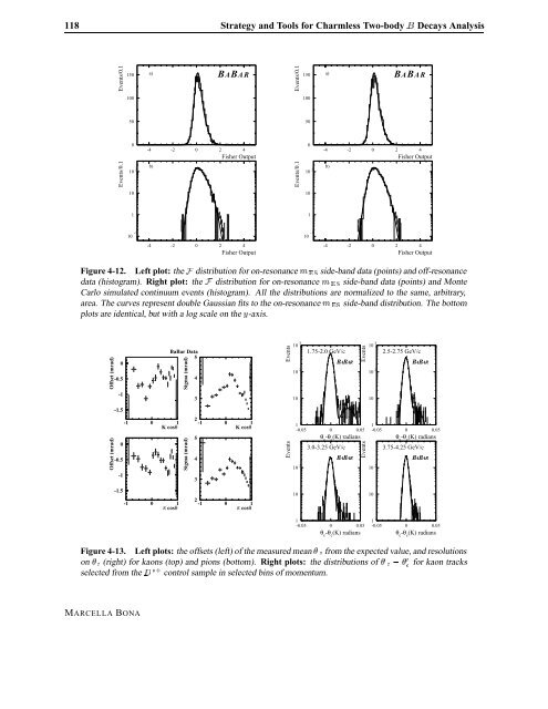
Page 123: 4.6 Analysis methods 117 Figure 4-1
Page 127 and 128: 5 Measurement of Branching Fraction
Page 129 and 130: 5.2 Ã Ë reconstruction 123 1 0.8
Page 131 and 132: 5.3 Analysis Strategy 125 0.35 0.3
Page 133 and 134: 5.4 Background Suppression and PDF
Page 139 and 140: 5.5 Maximum likelihood analysis 133
Page 151 and 152: 5.6 Counting analysis 145 Table 5-1
Page 153 and 154: 5.7 Determination of branching frac
Page 155 and 156: 6 Measurement of Branching Fraction
Page 157 and 158: 6.3 The maximum likelihood analysis
Page 163 and 164: 6.4 Counting analysis 157 120 100 8
Page 165 and 166: 6.5 Analysis choice 159 6.5 Analysi
Page 167 and 168: 6.6 Results on the Run1 data-set 16
Page 169 and 170: 6.7 Determination of the branching
Page 171 and 172: 7 Analysis of the time-dependent
Page 173 and 174: 7.3 Analysis strategy 167 Parameter
Page 175 and 176:
7.4 Data samples and event selectio
Page 177 and 178:
7.4 Data samples and event selectio
Page 179 and 180:
7.5 Background characterization 173
Page 181 and 182:
7.5 Background characterization 175
Page 183 and 184:
7.7 The maximum likelihood analysis
Page 185 and 186:
Page 187 and 188:
Page 189 and 190:
Page 191 and 192:
7.8 Validation studies 185 Figure 7
Page 193 and 194:
7.8 Validation studies 187 100 75 5
Page 195 and 196:
7.8 Validation studies 189 Figure 7
Page 197 and 198:
7.8 Validation studies 191 Paramete
Page 199 and 200:
7.9 Results 193 Parameter Fit Resul
Page 201 and 202:
7.9 Results 195 Events/2 MeV/c 2 Ev
Page 203 and 204:
7.10 Systematic studies 197 Categor
Page 205 and 206:
7.11 Summary 199 �Ã� Ë��
Page 207 and 208:
7.11 Summary 201 �Ã� Ë��
Page 209 and 210:
7.11 Summary 203 Variation �Ã�
Page 211 and 212:
BIBLIOGRAFIA 205 Bibliografia Chapt
Page 213 and 214:
BIBLIOGRAFIA 207 [38] J. Charles, P
Page 215 and 216:
BIBLIOGRAFIA 209 Chapter 7 [67] D.
show all

Violation in Mixing

You also want an ePaper? Increase the reach of your titles

Delete template?

Save as template?