Correction des exercices du livre La Gestion des Risques Financiers

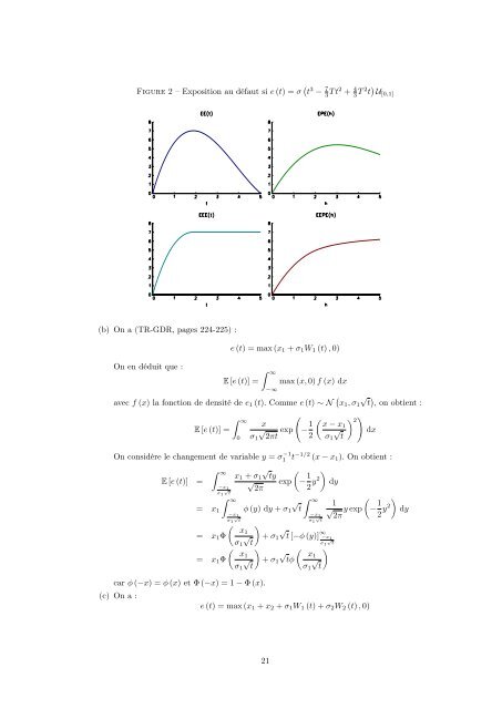
Figure 2 – Exposition au défaut si e (t) = σ ( t 3 − 7 3 T t2 + 4 3 T 2 t ) U [0,1](b) On a (TR-GDR, pages 224-225) :On en déduit que :e (t) = max (x 1 + σ 1 W 1 (t) , 0)E [e (t)] =∫ ∞−∞max (x, 0) f (x) dxavec f (x) la fonction de densité de e 1 (t). Comme e (t) ∼ N ( x 1 , σ 1√t), on obtient :E [e (t)] =∫ ∞−x 1σ 1√t∫ ∞0(x√ exp − 1 ( ) ) 2 x − x1√ dxσ 1 2πt 2 σ 1 tOn considère le changement de variable y = σ1 −1 t−1/2 (x − x 1 ). On obtient :E [e (t)] =exp(− 1 )2 y2 dyx 1 + σ 1√ty√2π∫ ∞ √∫ ∞= x 1 ϕ (y) dy + σ 1 t−x√ 1−x 1σ 1 t( )x1 √∞= x 1 Φ √ + σ 1 t [−ϕ (y)] −x1σ 1 t√σ 1 t= x 1 Φcar ϕ (−x) = ϕ (x) et Φ (−x) = 1 − Φ (x).(c) On a :σ 1√t1(x1σ 1√t)+ σ 1√tϕ(x1σ 1√t)√ y exp(− 1 )2π 2 y2e (t) = max (x 1 + x 2 + σ 1 W 1 (t) + σ 2 W 2 (t) , 0)dy21