- Page 1 and 2:
Wind Energy Proceedings of the Euro
- Page 3 and 4:
Prof. Dr. Joachim Peinke Dr. Stepha
- Page 5 and 6:
VI Preface been presented, spanning
- Page 7 and 8:
VIII Contents 3.3 Stochastic Wind F
- Page 9 and 10:
X Contents 12.6 Subgrid Scale Turbu
- Page 11 and 12:
XII Contents 22 Stochastic Small-Sc
- Page 13 and 14:
XIV Contents 32 Handling Systems Dr
- Page 15 and 16:
XVI Contents 41 3D Numerical Simula
- Page 17 and 18:
XVIII Contents 51 Comparing WAsP an
- Page 19 and 20:
XX Contents 58.3 Ultra-High Perform
- Page 21 and 22:
XXII List of Contributors Lars Berg
- Page 23 and 24:
XXIV List of Contributors Renata Gn
- Page 25 and 26:
XXVI List of Contributors A. Kiss D
- Page 27 and 28:
XXVIII List of Contributors El˙zbi
- Page 29 and 30:
XXX List of Contributors Ivo Sláde
- Page 31 and 32:
1 Offshore Wind Power Meteorology B
- Page 33 and 34:
1 Offshore Wind Power Meteorology 3
- Page 35 and 36:
1 Offshore Wind Power Meteorology 5
- Page 37 and 38:
2 Wave Loads on Wind-Power Plants i
- Page 39 and 40:
Trubaduren 2 Wave Loads on Wind-Pow
- Page 41 and 42:
Base moment (10 6 Nm) 0.4 0.2 −0.
- Page 43 and 44:
2 Wave Loads on Wind-Power Plants i
- Page 45 and 46:
3 Time Domain Comparison of Simulat
- Page 47 and 48:
3 Time Domain Comparison Using Cons
- Page 49 and 50:
7.0 6.0 5.0 4.0 3.0 2.0 1.0 0.0 3 T
- Page 51 and 52:
4 Mean Wind and Turbulence in the A
- Page 53 and 54:
4 Mean Wind and Turbulence in the A
- Page 55 and 56:
4 Mean Wind and Turbulence in the A
- Page 57 and 58:
5 Wind Speed Profiles above the Nor
- Page 59 and 60:
5 Wind Speed Profiles above the Nor
- Page 61 and 62:
Height [m] 100 90 80 70 60 50 40 30
- Page 63 and 64:
6 Fundamental Aspects of Fluid Flow
- Page 65 and 66:
f Suu(f, z) / σ 2 u(z) 10 0 10 −
- Page 67 and 68:
a) c) −0,375 6 Fluid Flow over Co
- Page 69 and 70:
7 Models for Computer Simulation of
- Page 71 and 72:
y/h 2.5 2 1.5 1 0.5 0 7 Models for
- Page 73 and 74:
8 Power Performance via Nacelle Ane
- Page 75 and 76:
8 Power Performance via Nacelle Ane
- Page 77 and 78:
8 Power Performance via Nacelle Ane
- Page 79 and 80:
9 Pollutant Dispersion in Flow Arou
- Page 81 and 82:
x1/B 0.3 0.5 0.8 1.0 9 Pollutant Di
- Page 83 and 84:
9 Pollutant Dispersion in Flow Arou
- Page 85 and 86:
10 On the Atmospheric Flow Modellin
- Page 87 and 88:
10 On the Atmospheric Flow Modellin
- Page 89 and 90:
10 On the Atmospheric Flow Modellin
- Page 91 and 92:
11 Comparison of Logarithmic Wind P
- Page 93 and 94:
Height above ground in m 100 90 80
- Page 95 and 96:
12 Turbulence Modelling and Numeric
- Page 97 and 98:
12 Turbulence Modelling and Numeric
- Page 99 and 100:
12 Turbulence Modelling and Numeric
- Page 101 and 102:
12 Turbulence Modelling and Numeric
- Page 103 and 104:
13 Gusts in Intermittent Wind Turbu
- Page 105 and 106:
13 Gusts in Intermittent Wind Turbu
- Page 107 and 108:
Durations (s) 25 20 15 10 5 13 Gust
- Page 109 and 110: 13 Gusts in Intermittent Wind Turbu
- Page 111 and 112: 14 Report on the Research Project O
- Page 113 and 114: height z (m) 100 80 60 40 20 0 14 R
- Page 115 and 116: 14.6 Outlook 14 Report on the Resea
- Page 117 and 118: 15 Simulation of Turbulence, Gusts
- Page 119 and 120: S(ƒ)(m/s) 2 /Hz 15 Simulation of T
- Page 121 and 122: 15 Simulation of Turbulence, Gusts
- Page 123 and 124: 16 Short Time Prediction of Wind Sp
- Page 125 and 126: ms prediction error [m/s] 16 Short
- Page 127 and 128: 16 Short Time Prediction of Wind Sp
- Page 129 and 130: 17 Wind Extremes and Scales: Multif
- Page 131 and 132: Log10 E(k)*k**(5/3) 6 4 2 0 5/3 cor
- Page 133 and 134: 17.3 Discussion and Conclusion 17 W
- Page 135 and 136: 18 Boundary-Layer Influence on Extr
- Page 137 and 138: z/H (a) (b) 4 2 18 Boundary-Layer I
- Page 139 and 140: 18.6 Concluding Remarks 18 Boundary
- Page 141 and 142: 19 The Statistical Distribution of
- Page 143 and 144: 19 The Statistical Distribution of
- Page 145 and 146: 20 Superposition Model for Atmosphe
- Page 147 and 148: h(u) 0.5 0.3 0.1 20 Superposition M
- Page 149 and 150: 21 Extreme Events Under Low-Frequen
- Page 151 and 152: 21 Extreme Events Under Low-Frequen
- Page 153 and 154: 22 Stochastic Small-Scale Modelling
- Page 155 and 156: p(σ⏐u) 1 0.8 0.6 0.4 0.2 22 Stoc
- Page 157 and 158: 22 Stochastic Small-Scale Modelling
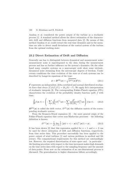
- Page 159: 23 Quantitative Estimation of Drift
- Page 163 and 164: 23 Quantitative Estimation of Drift
- Page 165 and 166: 24 Scaling Turbulent Atmospheric St
- Page 167 and 168: 24 Scaling Turbulent Atmospheric St
- Page 169 and 170: 25 Wind Farm Power Fluctuations P.
- Page 171 and 172: 25 Wind Farm Power Fluctuations 141
- Page 173 and 174: d rc q rc V 0 q V 25 Wind Farm Powe
- Page 175 and 176: References 25 Wind Farm Power Fluct
- Page 177 and 178: 26 Network Perspective of Wind-Powe
- Page 179 and 180: 26 Network Perspective of Wind-Powe
- Page 181 and 182: 26 Network Perspective of Wind-Powe
- Page 183 and 184: 27 Phenomenological Response Theory
- Page 185 and 186: 27 Phenomenological Response Theory
- Page 187 and 188: 27 Phenomenological Response Theory
- Page 189 and 190: 28 Turbulence Correction for Power
- Page 191 and 192: 28 Turbulence Correction for Power
- Page 193 and 194: 29 Online Modeling of Wind Farm Pow
- Page 195 and 196: 29 Online Modeling of Wind Farm Pow
- Page 197 and 198: 30 Uncertainty of Wind Energy Estim
- Page 199 and 200: 30 Uncertainty of Wind Energy Estim
- Page 201 and 202: 30 Uncertainty of Wind Energy Estim
- Page 203 and 204: 31 Characterisation of the Power Cu
- Page 205 and 206: 31 Characterisation of the Power Cu
- Page 207 and 208: 31 Characterisation of the Power Cu
- Page 209 and 210: 32 Handling Systems Driven by Diffe
- Page 211 and 212:
32 Handling Systems Driven by Diffe
- Page 213 and 214:
33 Experimental Researches of Chara
- Page 215 and 216:
33 Experimental Researches of Chara
- Page 217 and 218:
34 Methodical Failure Detection in
- Page 219 and 220:
34 Methodical Failure Detection in
- Page 221 and 222:
35 Modelling of the Transition Loca
- Page 223 and 224:
35 Modelling an Airfoil with Surfac
- Page 225 and 226:
(Cl/Cd)max 120 110 100 90 80 70 60
- Page 227 and 228:
35 Modelling an Airfoil with Surfac
- Page 229 and 230:
36 Helicopter Aerodynamics with Emp
- Page 231 and 232:
36 Helicopter Aerodynamics with Emp
- Page 233 and 234:
36 Helicopter Aerodynamics with Emp
- Page 235 and 236:
37 Determination of Angle of Attack
- Page 237 and 238:
37 Determination of Angle of Attack
- Page 239 and 240:
Drag coefficient 0.5 0.4 0.3 0.2 0.
- Page 241 and 242:
38 Unsteady Characteristics of Flow
- Page 243 and 244:
PSD PSD 38 Unsteady Characteristics
- Page 245 and 246:
39 Aerodynamic Multi-Criteria Shape
- Page 247 and 248:
39 Multi-Criteria Shape Optimizatio
- Page 249 and 250:
39 Multi-Criteria Shape Optimizatio
- Page 251 and 252:
40 Rotation and Turbulence Effects
- Page 253 and 254:
Cp Xsep/c 1 0.6 0.2 −0.2 −0.6
- Page 255 and 256:
Standard deviation of Cp 0.7 0.6 0.
- Page 257 and 258:
41 3D Numerical Simulation and Eval
- Page 259 and 260:
41 3D-CFD-Simulation of a Wind Turb
- Page 261 and 262:
42 Performance of the Risø-B1 Airf
- Page 263 and 264:
42 Performance of the Risø-B1 Airf
- Page 265 and 266:
43 Aerodynamic Behaviour of a New T
- Page 267 and 268:
43 Aerodynamic Behaviour of a New T
- Page 269 and 270:
43 Aerodynamic Behaviour of a New T
- Page 271 and 272:
44 Numerical Simulation of Dynamic
- Page 273 and 274:
44 Numerical Simulation of Dynamic
- Page 275 and 276:
45 Modeling of the Far Wake behind
- Page 277 and 278:
8 6 uz 4 2 45 Modeling of the Far W
- Page 279 and 280:
46 Stability of the Tip Vortices in
- Page 281 and 282:
46 Stability of the Tip Vortices in
- Page 283 and 284:
47 Modelling Turbulence Intensities
- Page 285 and 286:
47 Modelling Turbulence Intensities
- Page 287 and 288:
47 Modelling Turbulence Intensities
- Page 289 and 290:
48 Numerical Computations of Wind T
- Page 291 and 292:
Z X Y 48 Numerical Computations of
- Page 293 and 294:
References 48 Numerical Computation
- Page 295 and 296:
49 Modelling Wind Turbine Wakes wit
- Page 297 and 298:
U mean / U ref 1 0.9 0.8 0.7 49 Mod
- Page 299 and 300:
49.5 Conclusion 49 Modelling Wind T
- Page 301 and 302:
50 Prediction of Wind Turbine Noise
- Page 303 and 304:
0.8 0.6 0.4 0.2 −0.2 −0.4 −0.
- Page 305 and 306:
51 Comparing WAsP and Fluent for Hi
- Page 307 and 308:
Table 51.1. Measurements and simula
- Page 309 and 310:
51 Comparing WAsP and Fluent for Hi
- Page 311 and 312:
52 Fatigue Assessment of Truss Join
- Page 313 and 314:
52 Fatigue Assessment of Truss Join
- Page 315 and 316:
52 Fatigue Assessment of Truss Join
- Page 317 and 318:
53 Advances in Offshore Wind Techno
- Page 319 and 320:
Simulation Measurement pitch angle
- Page 321 and 322:
53 Advances in Offshore Wind Techno
- Page 323 and 324:
54 Benefits of Fatigue Assessment w
- Page 325 and 326:
∆σN [N/mm²] 100 10 54 Benefits
- Page 327 and 328:
55 Extension of Life Time of Welded
- Page 329 and 330:
Transverse residual stresses [N/mm
- Page 331 and 332:
56 Damage Detection on Structures o
- Page 333 and 334:
56 Damage Detection on Structures o
- Page 335 and 336:
57 Influence of the Type and Size o
- Page 337 and 338:
[W/m 2 ] q t [W/m 5000 4000 3000 20
- Page 339 and 340:
58 High-cycle Fatigue of “Ultra-H
- Page 341 and 342:
(a) (b) 450 Load [kN] 400 350 300 2
- Page 343 and 344:
59 A Modular Concept for Integrated
- Page 345 and 346:
59 A Modular Concept for Integrated
- Page 347 and 348:
59 A Modular Concept for Integrated
- Page 349 and 350:
60 Solutions of Details Regarding F
- Page 351 and 352:
SR 1000 800 600 400 200 100 80 60 4
- Page 353 and 354:
60 Solutions of Details Regarding F
- Page 355 and 356:
61 On the Influence of Low-Level Je
- Page 357 and 358:
Relative Power and Loading [%] 61 O
- Page 359 and 360:
62 Reliability of Wind Turbines Exp
- Page 361 and 362:
62 Reliability of Wind Turbines 331
- Page 363:
This page intentionally left blank


